Abstract: The Co-Creative Melody Generator is a system for simultaneous live coding with SuperCollider and OpenMusic. While in OpenMusic the music is created at note level, SuperCollider is responsible for sound generation. Communication takes place through the exchange of messages in the Open Sound Control protocol via user queries or automatically.
Responsible persons: Alexander Vozian
Overview:
The goal of the project was to integrate OpenMusic (OM) into a live coding workflow. My first idea was to use SuperCollider (SC) for sound generation and to outsource the setting of notes to OM. This means that you can code live in SC and use OM as an auxiliary tool. However, it became clear during the development that the OM patch can be changed in parallel during the sound output. As long as the sound-generating element is not interrupted, live coding can also take place in OM. For example, it is possible to prepare the selection of “instruments”, in this case SC synths, and control them completely in OM. Another more collaborative approach would be to split the two programs, SC and OM, between two live coders. For example, one person in SC could do the sound design, while another in OM sets these sounds in time.
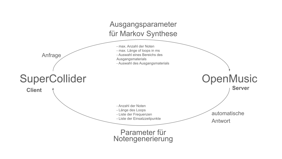
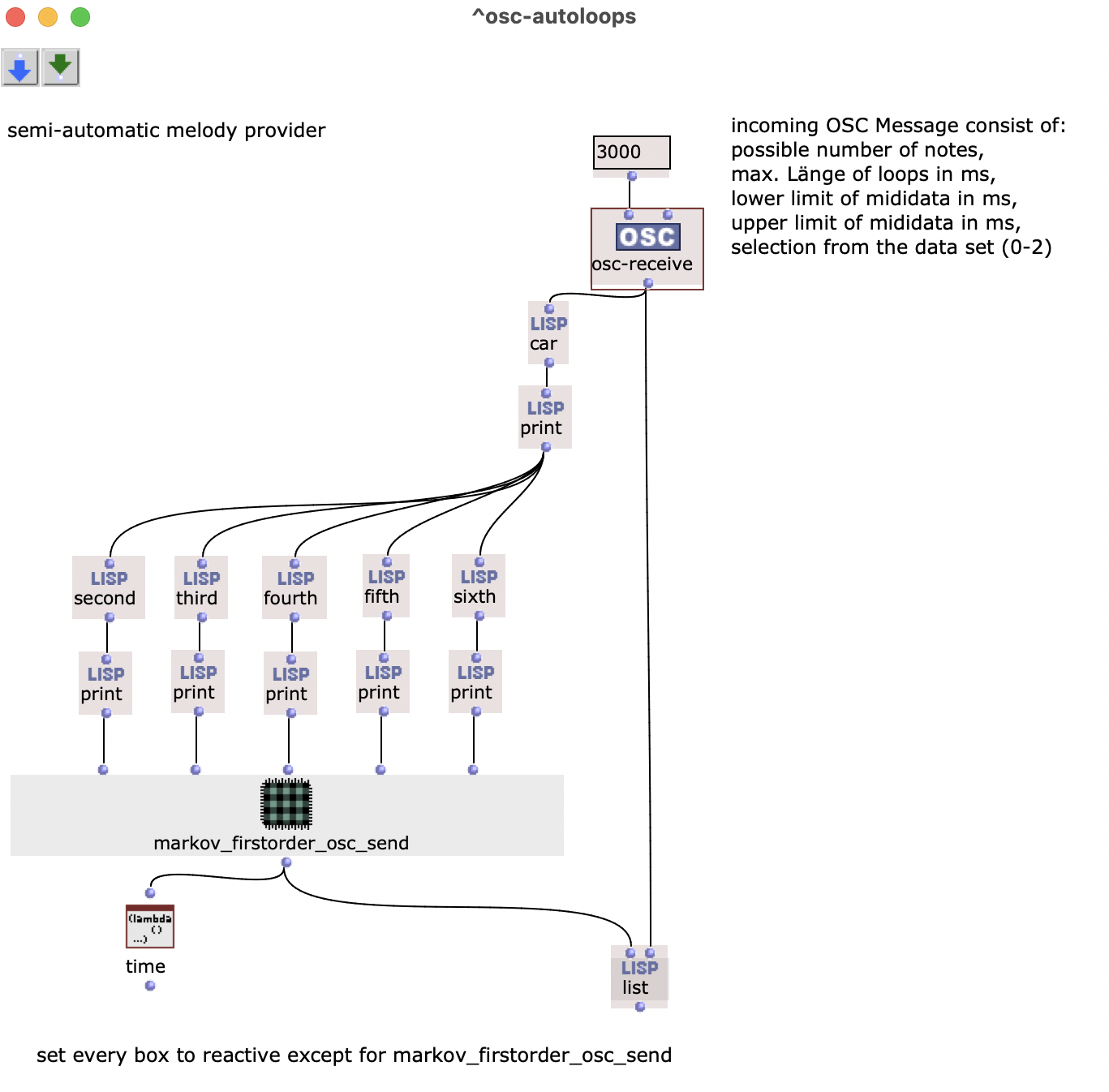
OM takes care of generating the notes and SC takes care of the sound synthesis. These communicate via the Open Sound Control (OSC) protocol. In SC, the user (live coder) sends a request to the OM patch via an OSC message. The message contains parameters for the generation of a melody, in this case for a Markov analysis and synthesis. The message consists of:
the maximum number of notes,
the maximum length of a loop in ms,
the lower and upper limit of the source material to be analyzed in ms
Selection of the source material.
The source material is a midi file, about 1 min long.
Sources of the midi files: bitmidi.com
After synthesis, OM automatically sends a message with the number of notes generated, the length of the melody in ms, a list of frequencies and a list of onsets. These are used to control the synths in SC.
With each evaluation, note material is analyzed and a list of frequencies and onsets is synthesized and then output.
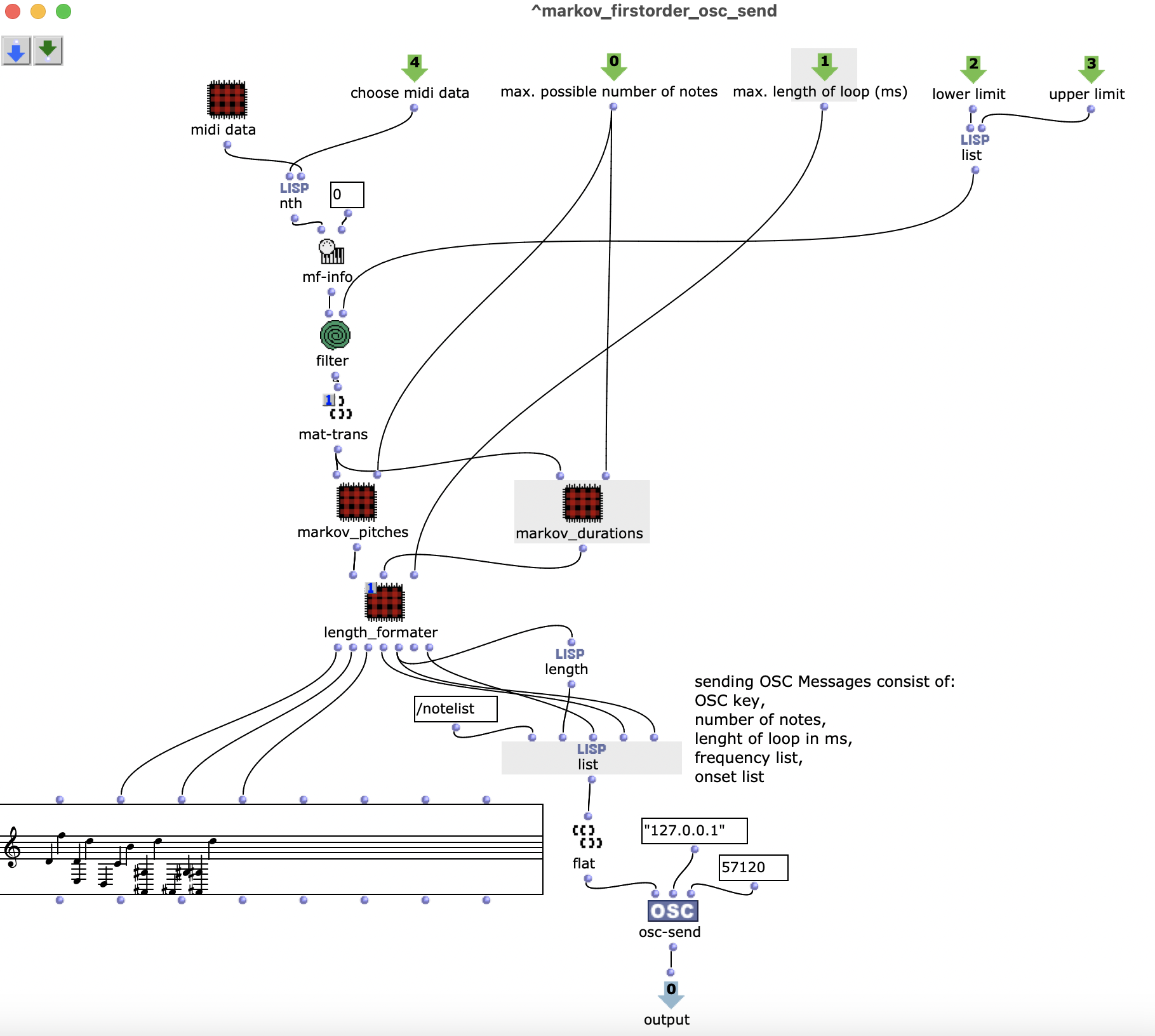
Midi files about 1 min long are used to generate the notes. The pitches and durations of the notes are analyzed independently of each other using first-order Markov functions from the OM-Alea library, synthesized and sent via osc-send. This results in tone sequences that do not occur in the original files. (The patch ensures that the list of pitches and durations is the same length) The input arguments are already described above.
An OSC message from OM to SC consists of the following data:
OSC Key as identifier,
Total number of notes,
Length of the melody in milliseconds,
List of frequencies,
List of onsets.
In this case, the total number of notes is only used to navigate through the unformatted OSC message. The length of the melody is required to determine the time at which the next melody is requested. The list of frequencies and onsets is only compiled in SC.
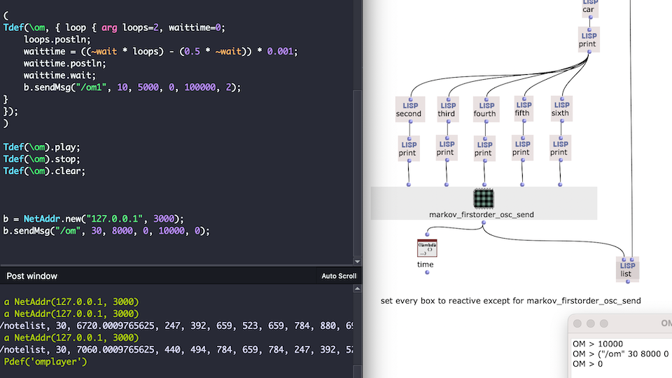
The osc-send function is in the patch markov_firstorder_osc_send. To execute the patch automatically when an OSC message arrives, all parts of the higher-level patch are set to reactive mode. The list function can only be evaluated when all forms deliver a result, i.e. when the Markov synthesis has been completed and osc-send has been executed.
The result is a kind of server that automatically sends back a melody when a request is received from SC.
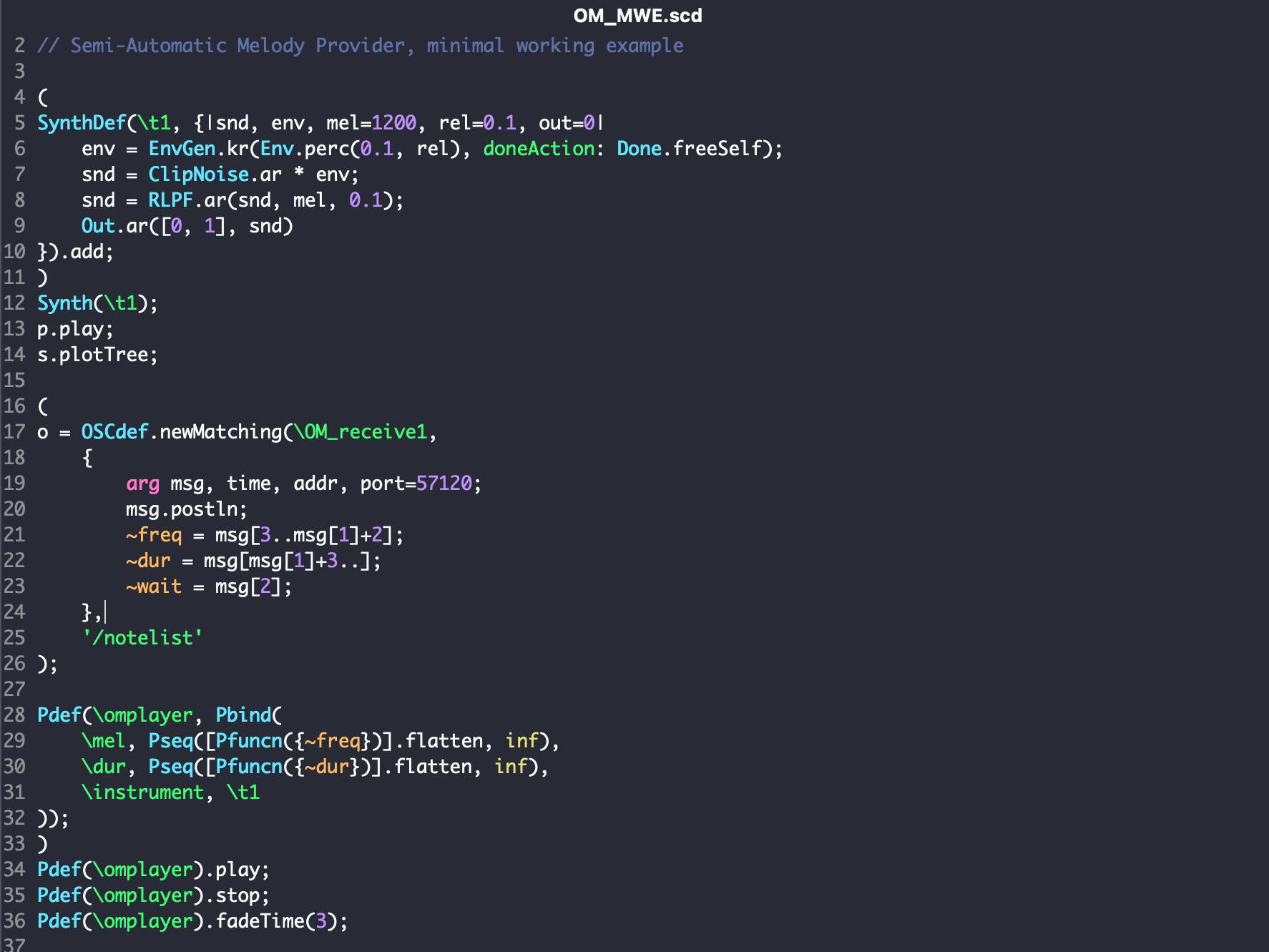
A new instance of OSCdef is created in SC, which saves the parameters received in global variables. A synth(t1) is defined that can be played by patterns. The Pfuncn function interprets the global variables ~freq and ~dur as functions and thus constantly queries them. The Pseq function converts these into a sequence, which is converted into a pattern by Pbind. Thus, the first parameter of ~freq with the first parameter of ~dur forms the first note of the melody. The Pdef function creates an instance that can be changed during runtime. This also ensures that a running loop only plays a new melody after the end of a melody.
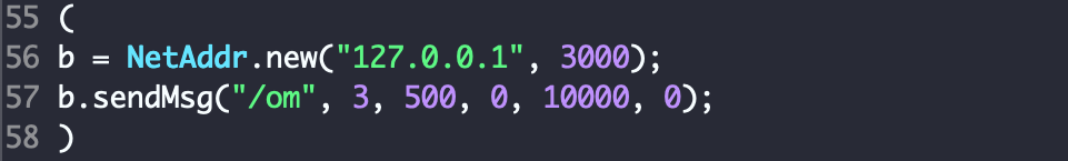
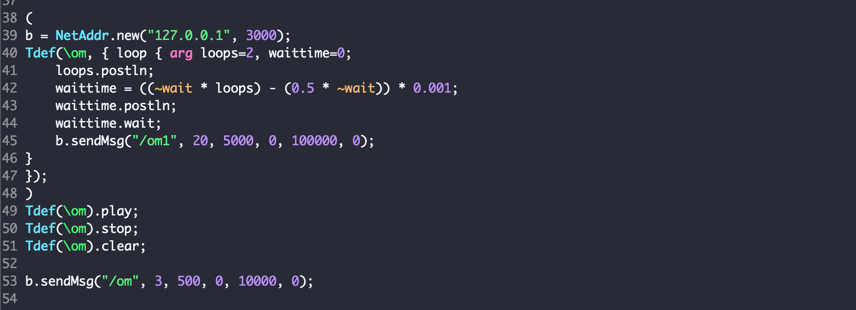
To request a new melody, a new loop, it is sufficient to send an OSC message with the corresponding parameters. To automate this process, you need the Tdef.
Just as the execution of a code block in SC can have a direct influence on the sound and must therefore be embedded correctly, the evaluation of a patch must take place at the right time. In the case of the MWE, it is not the sound that would be interrupted, but the meter.
Tdef(om) first calculates the time period with which the sending of the OSC message is delayed. The delay time depends on the total length of the loop and the number of loops that can be set within the Tdef. This ensures that the existing loop is always played to the end before the parameters for a new melody arrive.
The code for OM and SC can be found via this link.
Finally, the following sound example for the project:
Only the maximum length of a loop and the number of notes are changed. The source material is changed at two points. It starts with “Mario”, changes at around 1:39 to “Pokemon” and at 2:24 to “Tetris”. In the example, nothing is deliberately changed in the sound of the instrument (simple saw wave) in order to focus on the changes in the note material.
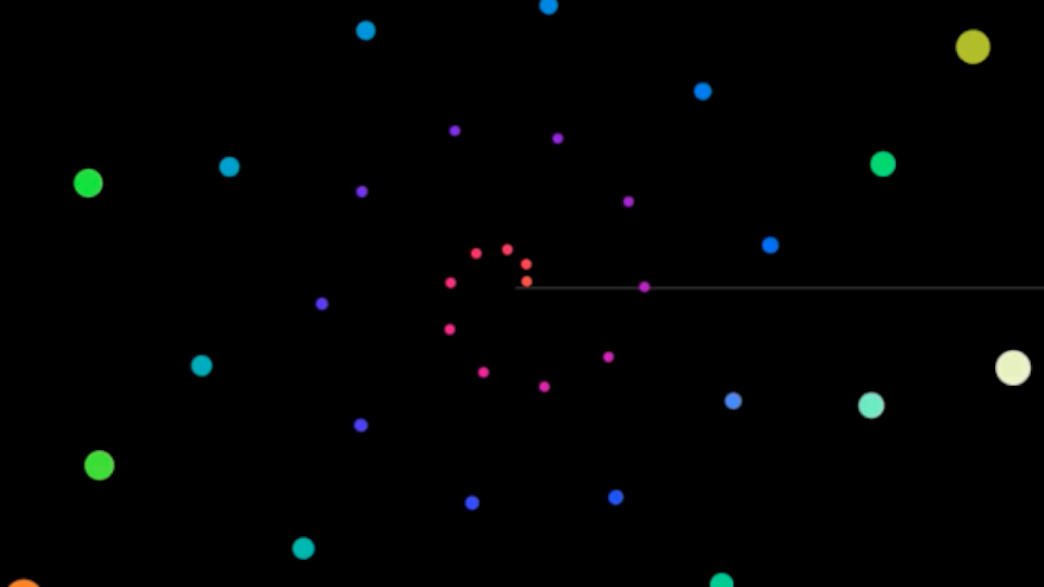
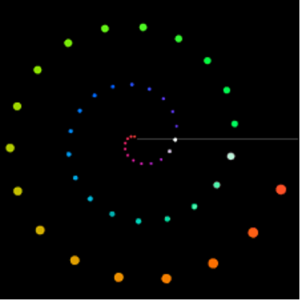
The Whitney Music Box is a sonified and/or visual representation of a series of interrelated sound elements. From a musical point of view, these elements can be related chromatically or harmonically, for example. In the visual representation, each of these elements is represented by a circle or dot (see Figure 1). These dots circle around a common center point depending on their own assigned frequency. The lower the frequency, the smaller the radius of the orbiting circle and the higher the orbital speed. Each sound element represents multiples of a fixed fundamental frequency in a harmonic series. As soon as an element has completed a revolution around the center point, the sound is triggered with the frequency it represents. Due to the mathematical relationship between the individual elements, there are moments during the performance of the Whitney Music Box in which certain elements are triggered simultaneously and phases in which the elements can be perceived consecutively. At the beginning and at the end, all elements are triggered simultaneously.
Figure 1: Whitney Music Box – visual representation
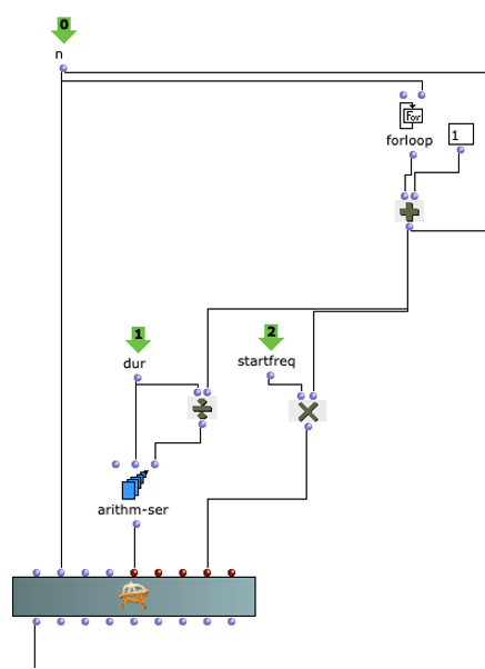
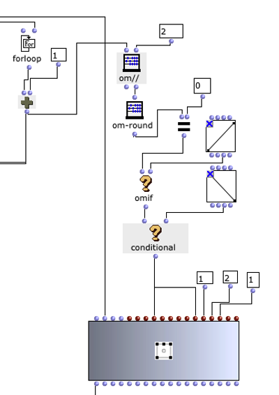
In this project, OMChroma is used to synthesize the individual sound elements (see Figure 2). The synthesis classes of OMChroma inherit from OpenMusic’s class-array object. The columns in the array describe the individual components within the synthesis. The rows represent parameters that can be assigned locally to the individual components or globally to the entire process. For the Whitney Music Box, elements are needed that implement the individual pitch gradations and the temporal offset of the individual pitch gradations. An OMChroma matrix is regarded as an event. Such an event represents a pitch and the sound repetitions within the global duration of the Whitney Music Box. The global duration is defined at the beginning and also describes the round trip time of the lowest frequency or the previously defined start frequency. Each matrix represents a frequency that is a multiple of the start frequency. The round trip time of a sound element is calculated using the formula
duration(global) / n
Where n is the index of the individual sound elements or matrices. The higher the index, the higher the frequency and the shorter the round trip time. The repetitions of the sound elements are defined by the parameter e-dels . Each component of a matrix is given a different entry delay. These entry delays are spaced at regular intervals of duration(global) / n.
Figure 2: Application of OMChroma
Without spatialization, the Whitney Music Box with OMChroma sounds like this:
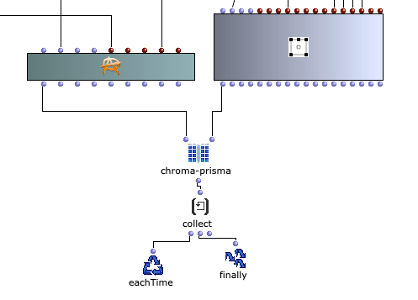
Figure 3 shows how the collected matrices or sound events are spatialized with the OMPrisma library. This was based on the visual representation of the Whitney Music Box. Sound elements with a low frequency are further away from the center and sound elements with a high frequency circle closer to the center. With OMPrisma, this representation is to be implemented in spatial sound. This means that sounds with a low frequency should sound further away and sounds with a high frequency should sound closer to the listener. In the OpenMusic patch, elements with an even index were also positioned further to the front and further to the right and, similarly, elements with an odd index were positioned further to the left and back in order to distribute the sounds evenly in the room. The OMPrisma classes also offer presets for the attenuation function, air-absorption function and time-of-flight function . These were used to create an even greater sense of spatiality in addition to the positioning in the room.
Figure 3: Application of OMPrisma
In stereo, for example, the Whitney Music Box sounds like this:
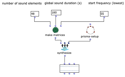
Figure 4 shows how the collected OMChroma and OMPrisma matrices are merged using the chroma-prisma function. The list of all collected matrices is returned via an om-loop and rendered as a sound using the synthesize function(see Figure 5).
This article is about the fourth iteration of an acousmatic study by Zeno Lösch, which was carried out as part of the seminar “Visual Programming of Space/Sound Synthesis” with Prof. Dr. Marlon Schumacher at the HFM Karlsruhe. The basic conception, ideas, iterations and the technical implementation with OpenMusic will be discussed.
Responsible persons: Zeno Lösch, Master student Music Informatics at HFM Karlsruhe, 2nd semester
Pixel
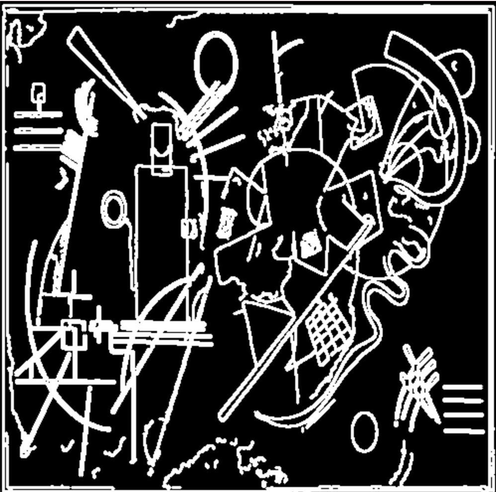
A Python script was used to obtain parameters for modulation.
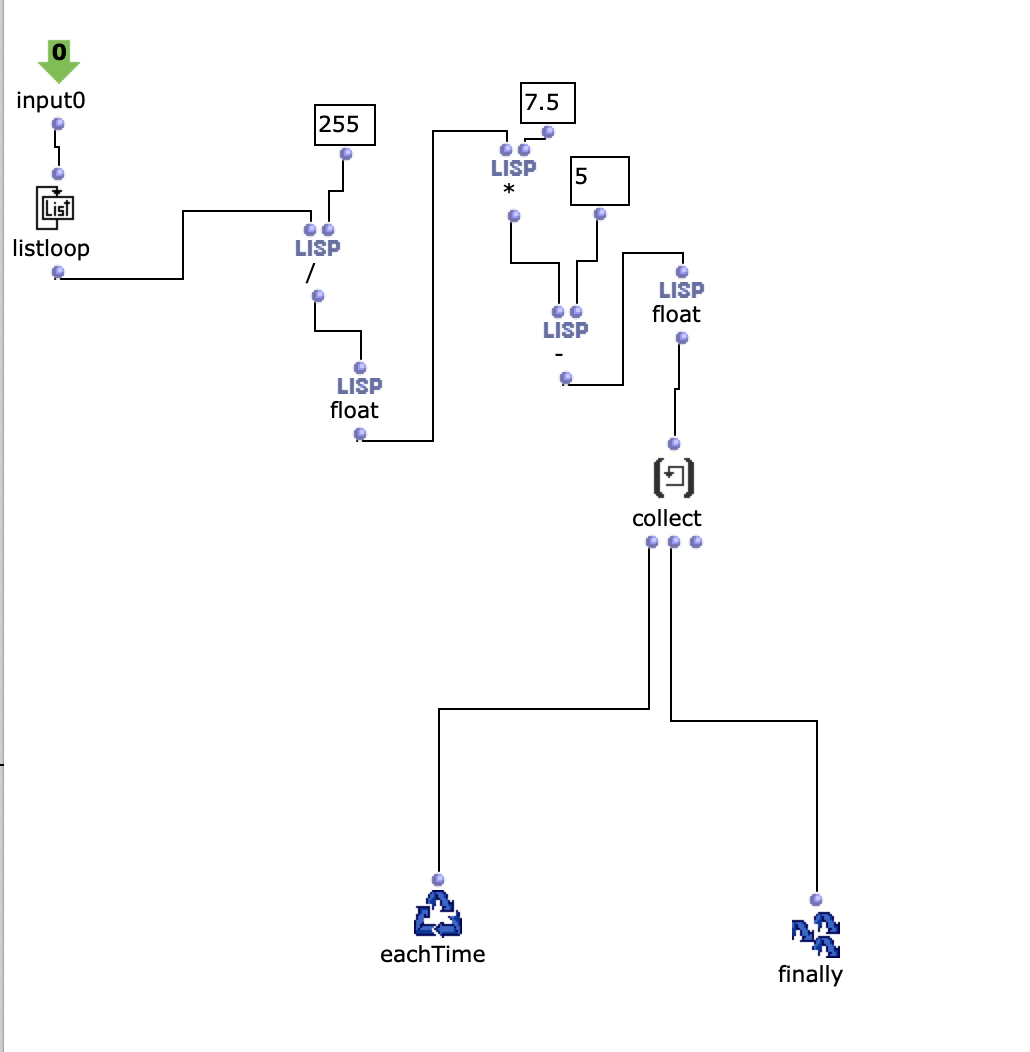
This script makes it possible to scale any image to 10 x 10 pixels and save the respective pixel values in a text file. “99 153 187 166 189 195 189 190 186 88 203 186 198 203 210 107 204 143 192 108 164 177 206 167 189 189 74 183 191 110 211 204 110 203 186 206 32 201 193 78 189 152 209 194 47 107 199 203 195 162 194 202 192 71 71 104 60 192 87 128 205 210 147 73 90 67 81 130 188 143 206 43 124 143 137 79 112 182 26 172 208 39 71 94 72 196 188 29 186 191 209 85 122 205 198 195 199 194 195 204 ” The values in the text file are between 0 and 255. The text file is imported into Open Music and the values are scaled.
These scaled values are used as pos-env parameters.
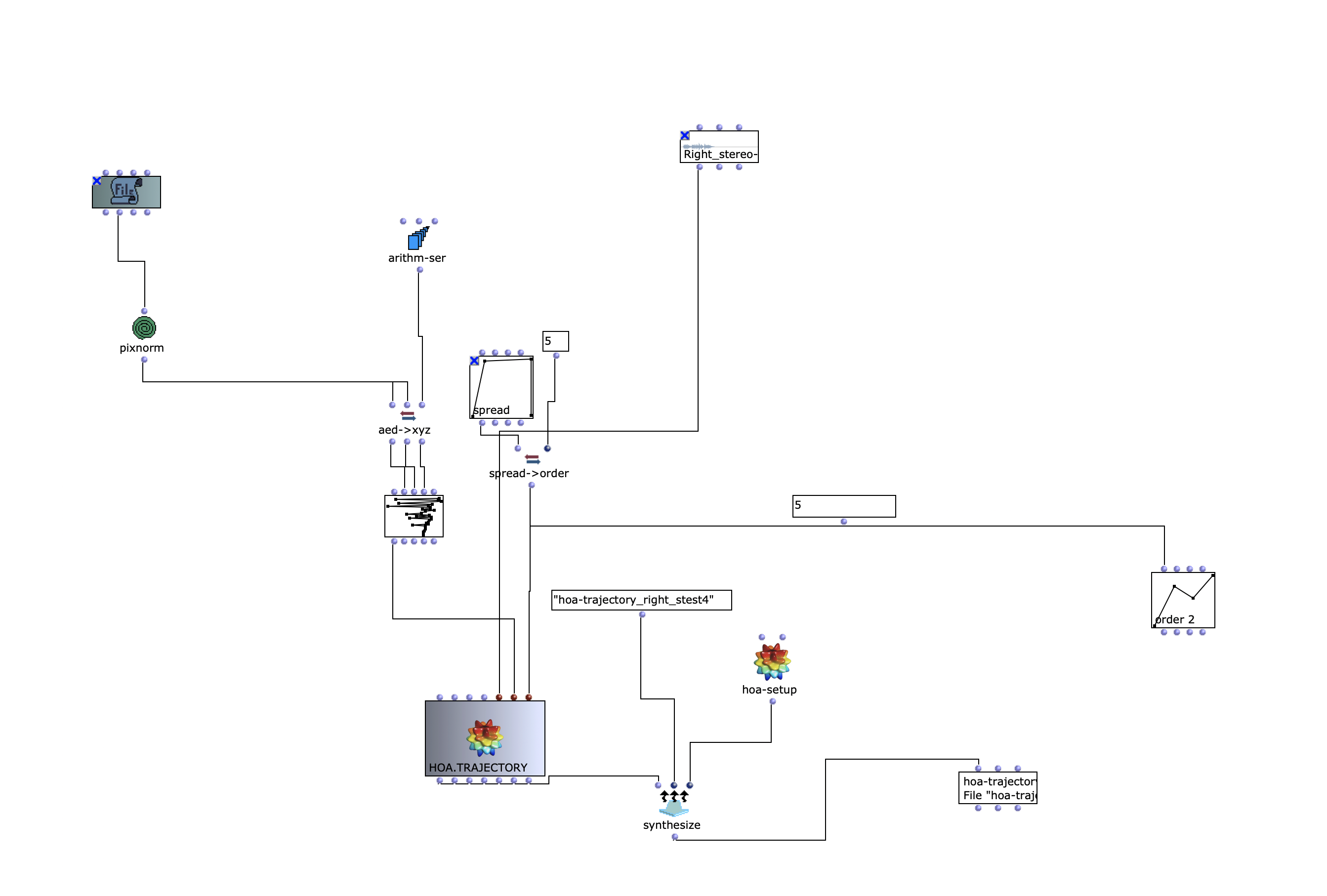
Reaper and IEM-Plugin Suite
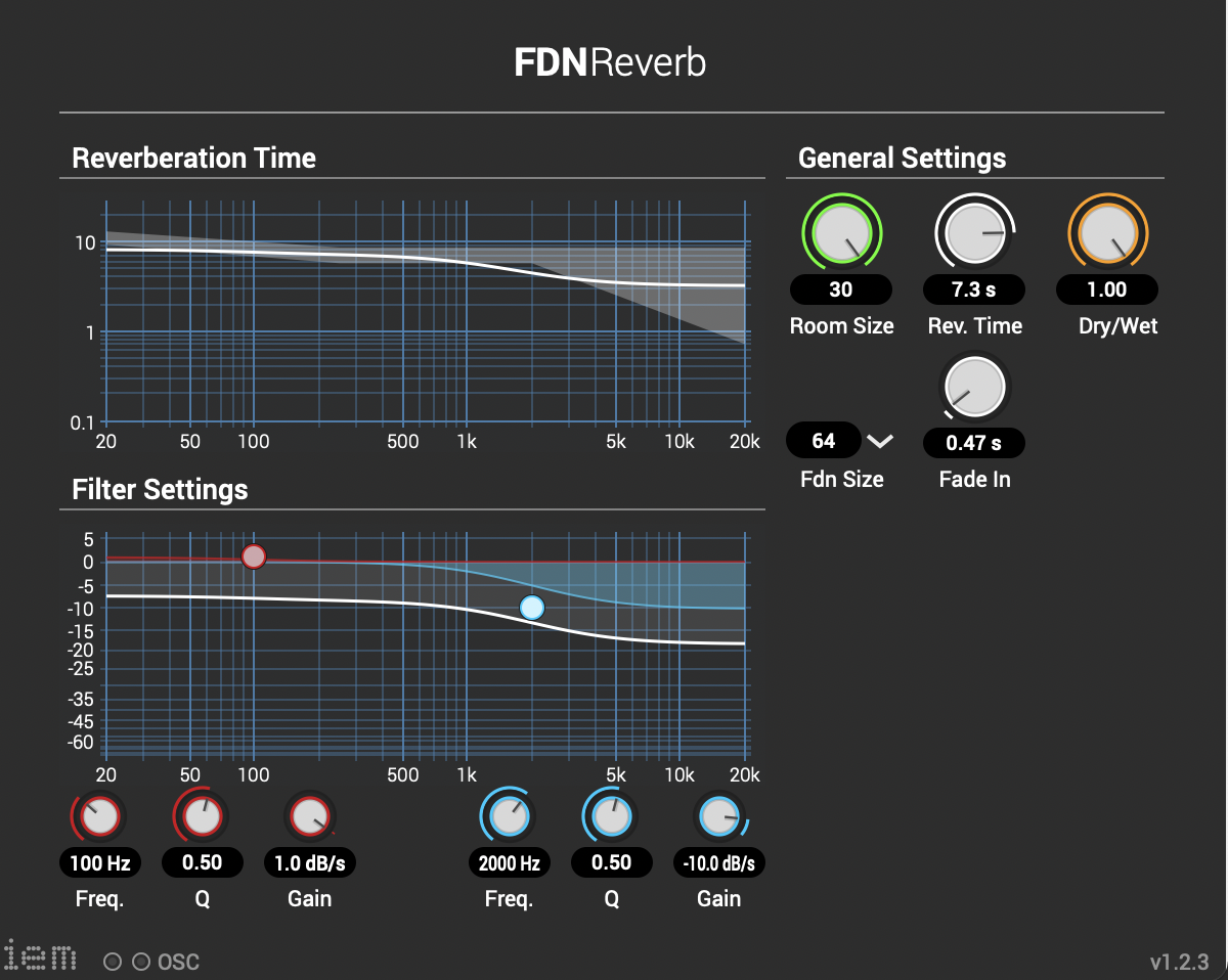
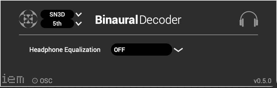
With different images and different scaling, you get different results that can be used as parameters for modulation. In Reaper, the IEM plug-in suite was used in post-production. These tools are used for Ambisonics of different orders. In this case, Ambisonics 5 order was used. One effect that was often used is the FDNReverb. This reverb unit offers the possibility of applying an Ambisonics reverb to a multi-channel file. The stereo and mono files were first encoded in 5th order Ambisonics (36 channels) and then converted into two channels using the binaural encoder. Other post-processing effects (Detune, Reverb) were programmed by myself and are available on Github. The reverb is based on a paper by James A. Moorer About this Reverberation Business from 1979 and was written in C. The algorithm of the detuner was written in C from the HTML version of Miller Puckette’s handbook “The Theory and Technique of Electronic Music”. The result of the last iteration can be heard here.
A link to download the applications can be found at the end of this blogpost. This project was also presented as a paper at the 2022 International Conference on Technologies for Music Notation and Representation (TENOR 2022).
Modularity in Sound Synthesis Tools
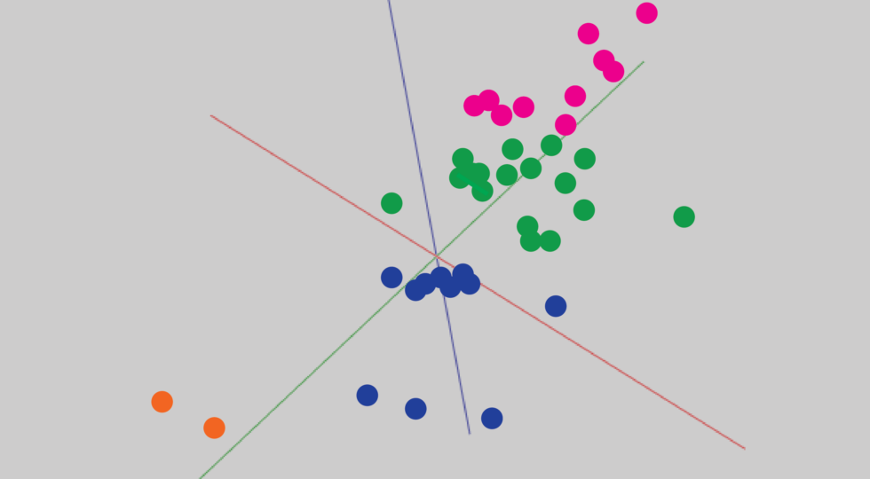
This blogpost walks through the structure and usage of two applications of machine learning (ML) methods for sound notation and synthesis. The first application is a modular sample replacement engine that uses a supervised classification algorithm to segment and transcribe a drum beat, and then reconstruct that same drum beat with different samples. The second application is a texture synthesis engine that uses an unsupervised clustering algorithm to analyze and sort large numbers of audio files.
The applications were developed in OpenMusic using the OM-SoX modular synthesis/analysis framework. This was so that the applications could be as modular as possible. Modular, meaning that they could be customized, extended, and integrated into a user’s own OpenMusic workflow. We believe this modularity offers something new to the community of ML and sound synthesis/analysis tools currently available. The approach to sound synthesis and analysis used here involves reading and querying many separate audio files. Such an approach can be encompassed by the larger term of “corpus-based concatenative synthesis/analysis,” for which there are already several effective tools: the Caterpillar System, Audioguide, and OM-Pursuit. Additionally, OM-AI, ml.*, and zsa.descriptors are existing toolkits that integrate ML methods into Computer-Aided Composition (CAC) environments. While these tools are very precise, the internal workings of them are not immediately clear. By seeking for our applications to be modular, we mean that they can be edited, extended and integrated into existing CAC programs. It also means that they can be opened and up, examined, and reverse-engineered for a user’s own education.
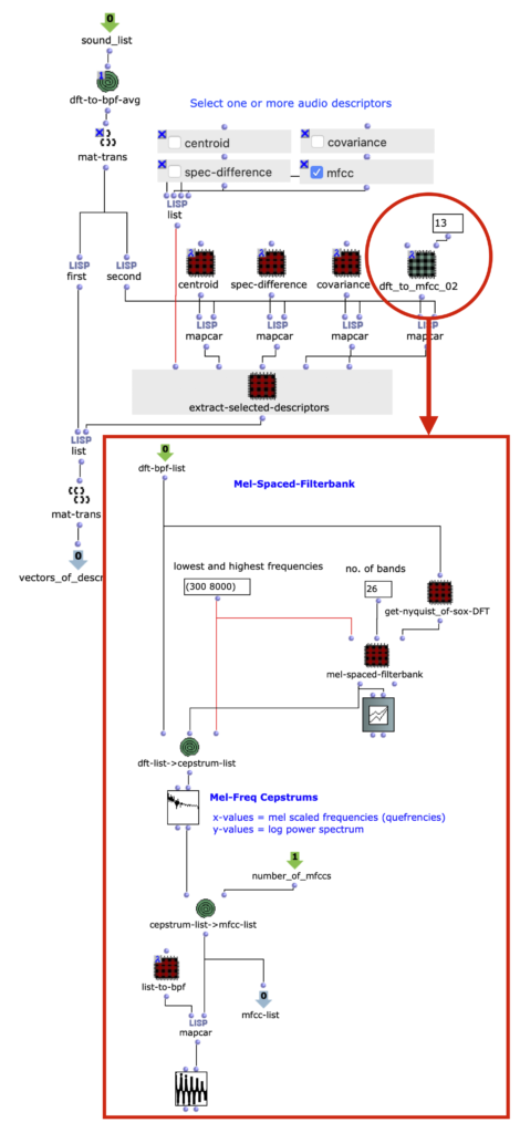
One example of this is in figure 1, our audio analysis engine. Audio descriptors are implemented as subpatches in lambda mode, and can be selected as needed for the input audio.
Figure 1: Interchangeable audio descriptors are set as patches in lambda mode. Here, a patch extracting 13 MFCCs is being used.
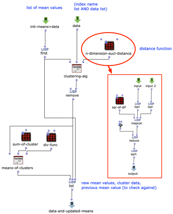
Another example is in figure 2, a customizable distance function in our texture synthesis application. This is the ML clustering algorithm that drives the application. Being a patch built from smaller OpenMusic objects, it is not only a tool for visualizing the algorithm at work, it also allows a user to edit it. For example, the n-dimension euclidean distance function could be substituted with another distance function, if needed.
Figure 2: A simple k-means clustering algorithm, built within an OpenMusic abstraction. The distance function takes the form of a subpatcher in lambda mode.
With the modularity of the project introduced, we will on the next page move on to the two specific applications.
Up until this past August, my impressions of what machine learning could be used for was mostly functional, detached from any aesthetic reference point within my artistic practice. Cars recognizing stop signs, radiologists detecting malignant legions in tissue; these are the first things to come to my mind. There is definitely an art behind programming these tasks. However, it wasn’t clear to me yet how machine learning could relate to my world of contemporary concert music. Therefore, when I participated in Artemi-Maria Gioti’s machine learning workshop at impuls Academy 2021, my primary interest was to make personal artistic connections to this body of research, and to see what ways I could interrogate my underlying aesthetic assumptions in artistic applications of machine learning. The purpose of this text is to share with you the connections I made. I will walk through the composition process of my piece Shepherd for voice and live electronics, using it as a frame to touch upon basic machine learning theories and methods, as well as outline how I aesthetically reacted to them. I will not go deep into the technicalities of machine learning – there are far more qualified people than I for that specific task. However, I will say that the technical content of this blogpost is inspired heavily from Artemi-Maria Gioti, who led this workshop and whose research covers the creative applications of machine learning in a much deeper way. A further dive into the already rich world of machine learning and music can be begun at her website.
A fundamental definition of machine learning can be framed around the idea of improvement through experience. As computer scientist Tom M. Mitchell describes it, “The field of machine learning is concerned with the question of how to construct computer programs that automatically improve with experience.” (Mitchell, T. (1998). Machine Learning. McGraw-Hill.). This premise of ‘improvement’ already confronted me with non-trivial questions. For example, if machine learning is utilized to create an improvising duo partner, what exactly does the computer understand as ‘good’ or ‘bad’ improvisation, as it gains experience? Before even beginning to build a robust machine learning algorithm, answering this preliminary question is an entire undertaking in and of itself. In my piece Shepherd, the electronics were trained to recognize the sound of my voice, specifically whether I was whispering, talking, yelling, or being silent. However, my goal was not to create a perfectly accurate recognition algorithm. Rather, I wanted the effectiveness and the ineffectiveness of the algorithm to both play equal roles in achieving the piece’s concept. Shepherd is a performance piece takes after a metaphor from Jesus in the christian bible – sheep recognize a shepherd by the sound of their voice (John 10). The electronics reacts to my voice in a way that is simultaneously certain and uncertain. It is a reflection, through performance, on the nuances of spiritual faith, the way uncertainty necessarily partakes in the formation of conviction and belief. Here the electronics were not functional instrument (something designed to be controlled by my voice), but rather were functioning more as a second player (a duo partner, reacting to my voice with a level of unpredictability).
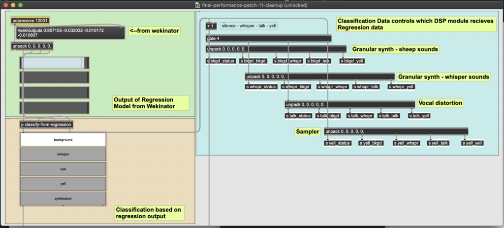
Concretely in the program, the electronics returned two separate answers for every input it is given (see figure 1). It gives a decisive, classification answer (“this is ‘silence’, this is ‘whispering’, this is ‘talking’, etc.), and it gives an indecisive, erratic answer via regression (‘silence: 0.833; whispering: 0.126; talking: 0.201; yelling: 0.044’). And important for this concept of conceiving belief through doubt, the classification answer is derived from the regression answer. The decisive answer (classification) was generally stable in its changes over time, while the indecisive answer (regression) moved more quickly and erratically. Overall, this provided a useful material for creating dynamic control of the actual digital sounds that the electronics produced. But before touching on the DSP, I want to outline how exactly these machine learning algorithms operate, how the electronics learn and evaluate the sound of my voice.
Figure 1: Max MSP and Wekinator (off-screen) analyze an audio’s MFCCs to give two outputs on the nature of the input audio. The first output is from a regression algorithm, the second is from a classification algorithm.
In order for the electronics to evaluate my input voice, it first needs a training set, a collection of data extracted from audio of my voice, with which it could use to ‘learn’ my voice. An important technical point is that the machine learning algorithm never observes actual audio data. With training and testing data, the algorithm is always looking at numerical data (here called ‘descriptors’) extracted from the audio. This is one reason machine learning algorithms can work in realtime, even with audio. As I alluded to, my voice recognition program is underpinned by two machine learning concepts: classification and regression. A classification algorithm will return a discrete value from its input data. In my case, those values are ‘silence’, ‘whispering’, ’talking’, and ‘yelling’. To make a training set then, I recorded audio of each of these classes (4 audio files in total), and extracted MFCCs (Mel-Frequency Cepstrum Coefficients) from it. MFCC’s are a representation a sound’s spectral energy calibrated to the range of typical human auditory perception, and are already commonly used in speech recognition programs, music-information retrieval applications, and other applications based around timbre-recognition.
I used the Max MSP library Zsa.descriptors to calculate my MFCCs. I also experimented with other audio descriptors such as spectral centroid, spectral flatness, amplitude peaks, as well as varying numbers of MFCC’s. Eventually I discovered that my algorithm was most accurate when 13 MFCCs were the only descriptor, and that description data was taken only about fivetimes a second. I realized that, on a micro-level timescale, my four classes had a lot similarity. For example, the word ‘synthesizer,’ carried lots of ’s’ noise, which is virtually the same when whispered as when talked. Because of this, extracting data at an intentionally slower rate gave the algorithm a more general picture of each of my voice-classes, allowing these micro-moments of similarity to be smoothed out.
The standard algorithm used for my voice recognition concept was classification. However, my classification algorithm was actually built using a second common machine learning algorithm: regression. As I mentioned before, I wanted to build into my electronics a level of ‘indecision’, something erratic that would contrast the stable nature of a standard classification algorithm. Rather than returning discrete values, a regression algorithm gives a new ‘predictive’ value, based on a function derived from the training set data. In the context of my piece, the regression algorithm does not return a specific voice-class. Rather, it gives four percentage values, each corresponding to how close or far my input is to each of the four voice-classes. Therefore, though I may be whispering, the algorithm does not say whether I am whispering or not. It merely tells me how close or far away I am from the ‘whispering’ data that it has been trained on.
I used a regression algorithm in Wekinator, a simple and powerful machine learning tool, to build my model (see figure 2). Input audio was analyzed in Max MSP, and the descriptor data was sent via OSC to Wekinator. Wekinator built the predictive regression model from this data and then sent output back to Max MSP to be used for DSP control. In Max, I made my own version of a classification algorithm based on this regression data.
Figure 2: Wekinator is evaluating MFCC data from Max MSP and returning 4 values from 0.0-1.0, indicating the input’s similarity to the four voice classes (silence, whispering, talking, yelling). The evaluation is a regression model trained on 752 data samples.
All this algorithm-building once again returns me to my original concern. How can I make an aesthetic connection with these concepts? As I mentioned, this piece, Shepherd is for my solo voice and live electronics. In the piece I stand alone on a stage, switching through different fictional personas (a speaker at a farming convention, a disgruntled restaurant chef, a compilation video of Danny Wolfers saying the word ‘synthesizer,’ and a preacher), and the electronics reacts to these different characters by switching through its own set of personas (sheep; a whispering, whimpering sous chef; a literal synthesizer; and a compilation of christian music). Both the electronics and I change our personas in reaction to each other. I exercise some level control over the electronics, but not total. As I said earlier, the performance of the piece is a reflection on the intertwinement of conviction and doubt, decision and indecision, within spiritual faith. Within this concept, the idea of a machine ‘improving’ towards ‘perfection’ is no longer an effective framework. In the concept, and consequently in the music I attempted to make, stable belief (classification) and unstable indecision (regression) were equal contributors towards the musical relationship between myself and the electronics.
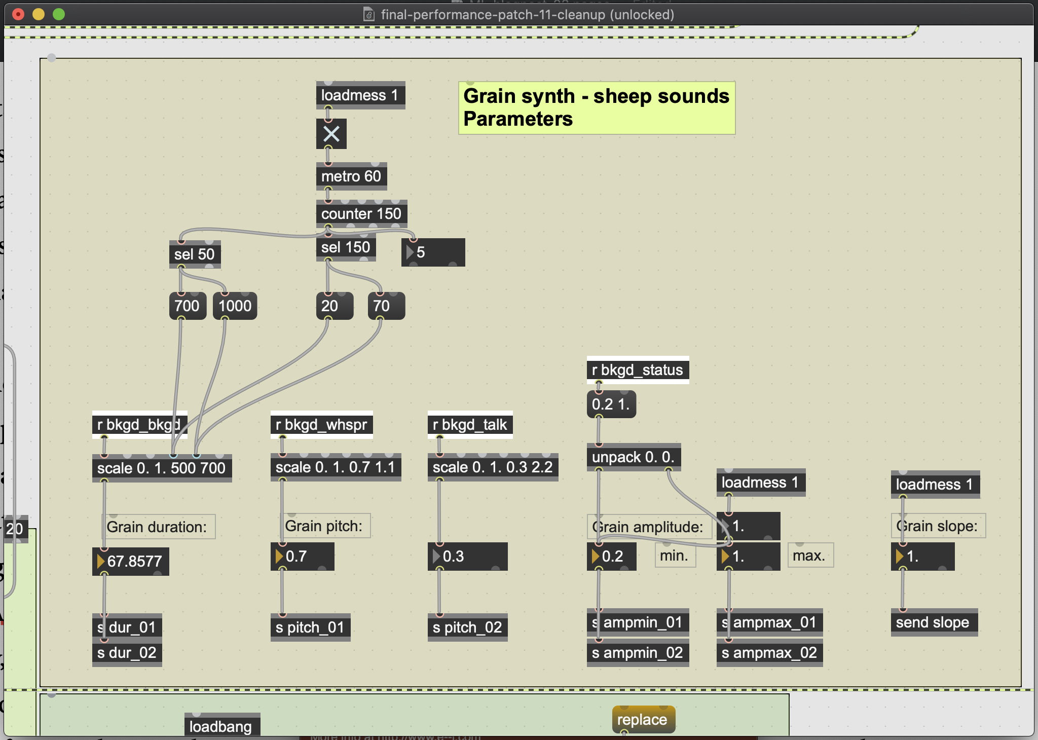
Based on how my voice was classified, the electronics operated one of four DSP modules. The individual parameters of a given module were controlled by the erratic output data of the regression algorithm (see figure 3). For example, when my voice was classified as silent, a granular synthesizer would create textures of sheep-like noises. Within that synthesizer, the percentage levels of whispering and talking ‘detected’ within the silence would manipulate the pitch shifting in the synthesizer (see figure 4). In this way, the music was not just four distinct sound modules. The regression algorithm allowed for each module to bend and flex in certain directions, as my voice subtly suggested hints of one voice class from within another. For example, in one section I alternate rapidly between the persona of a farmer talking at a farming convention, and a chef frustratingly whispering at his sous chef. The electronics moved consequently between my whispering and talking DSP modules. But also, as my whispering became more frustrated and exasperated, the electronics would output higher levels of talking in its regression algorithm. Thus, the internal drama of my theatricalperformances is reacted to by the electronics.
Figure 3: The classification data would trigger one of four DSP modules. A given DSP module would receive the regression values for all four vocal classes. These four values would control the parameters of the DSP module.
Figure 4: Parameter window for granular synth triggered when the electronics classifies my voice as ‘silent’. The amount of whispering and talking detected in the silence would control the pitch of the grain. The amount of silence detected in the silence controlled the grain’s duration. Because this value is relatively static during actual silence from my voice, a level of artificial duration manipulation (seen a the top of the window) was programmed.
I want to return to Tom Mitchell’s thesis that machine learning involves computer improvingautomatically through experience. If Shepherd is a voice recognition tool, then it is inefficient at improvement. However, Shepherd was not conceived as a tool. Rather, creating Shepherd was more so a cultivation of a relationship between my voice and the electronics. The electronics were more of a duo partner, and less of an instrument. To put this more concretely, I was never looking for ‘accurate’ results from the machine. As I programmed, I was searching for results that illustrated Shepherd’s artistic concept of belief intertwined with doubt. In this way, ‘improving’ the piece did not mean improving the algorithm’s accuracy. It meant ‘improving’ the relationship between myself and the electronics. One positive from this approach is that the compositional process was never separated from the programming of the electronics. Both developed in tandem. The composing this piece brought me to the realization that creative applications of machine learning can be applied at every level of its discourse. If you ware interested in hearing a recording of this performance, a bootleg recording of the premiere can be found here.
https://youtu.be/LFQnpp5Uzbg
References:
Artemi-Maria Gioti – composer and artistic researcher working in the field of artificial intelligence.
Wekinator – free, open-source software created by Rebecca Fiebrink that uses machine learning to create musical instruments, game interfaces, computervision, and other tools in sound and animation.
Zsa.descriptors – library for real-time sound descriptors analysis for Max MSP developed by Mikhail Malt and Emmanuel Jourdan.

 The stereo and mono files were first encoded in 5th order Ambisonics (36 channels) and then converted into two channels using the binaural encoder.
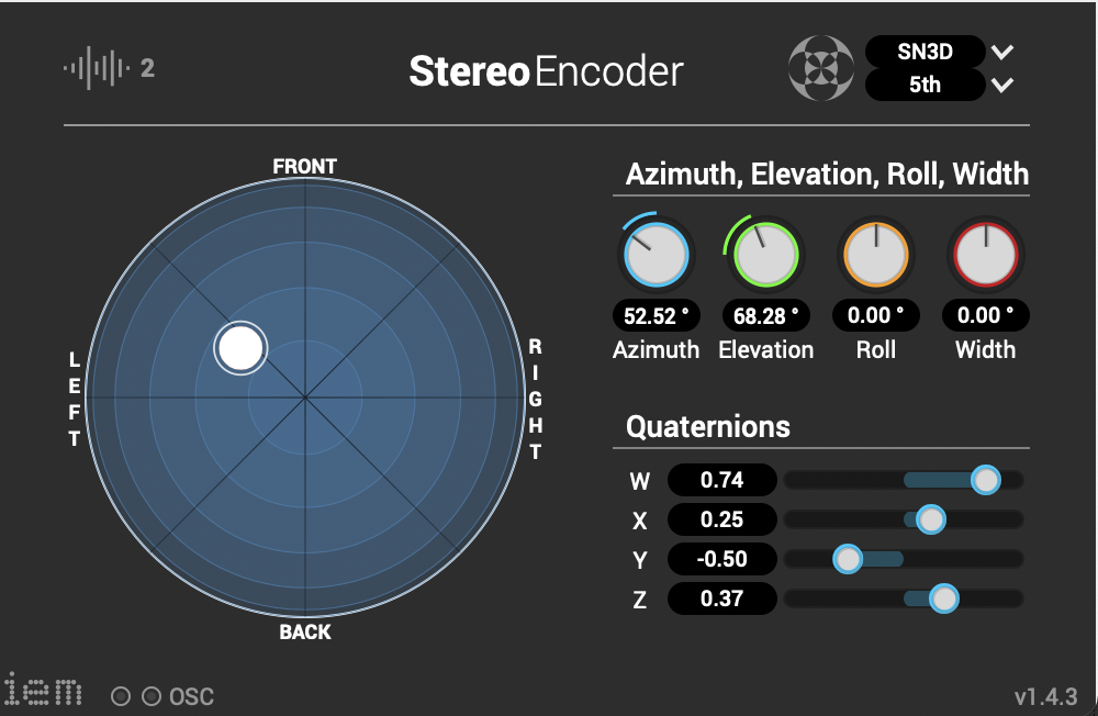
 Other post-processing effects (Detune, Reverb) were programmed by myself and are available on Github. The reverb is based on a paper by James A. Moorer About this Reverberation Business from 1979 and was written in C. The algorithm of the detuner was written in C from the HTML version of Miller Puckette’s handbook “The Theory and Technique of Electronic Music”. The result of the last iteration can be heard here.