We present an approach to geometrically represent and analyze the harmonic content of musical compositions based on a formalization of chord sequences as spatial trajectories. This allows us in particular to introduce a toolbox of novel descriptors for automatic music genre classification. Our analysis method first of all implies the definition of harmonic trajectories as curves in a type of geometric pitch class spaces called Tonnetz. We define such curves by representing successive chords appearing in chord progressions as points in the Tonnetz and by connecting consecutive points by geodesic segments. Following a recently established hypothesis that assumes the existence of a narrow link between the musical genre of a work and specific geometric properties of its spatial representation, we introduce a toolbox of descriptors relating to various geometric aspects of the harmonic trajectories. We then assess the appropriateness of these descriptors as a classification tool that we test on compositions belonging to different musical genres. In a further step, we define a representation of transitions between two consecutive chords appearing in a harmonic progression by vectors in the Tonnetz. This allows us to introduce an additional classification method based on this vectorial representation of chord transitions.
Abstract: The OpenMusic program PixelWaltz can be used to convert images into symbolic representations of music (pitches and onset times). Options for image manipulation are available with which the result can be additionally influenced.
Responsible persons: Florian Simon
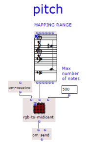
Mapping: Pitch
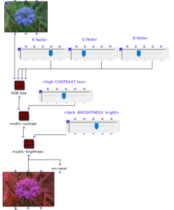
The pixels of the image are scrolled through line by line and the respective red, green and blue values (between 0 and 1) are mapped to a desired pitch range. This means that three pitch values in midicent are always obtained from one pixel. As two adjacent pixels are similar in many cases, this mapping method often results in repeating patterns every three notes. This is the reason for the title of the project.
It is also possible to limit the number of note values output.
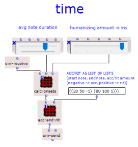
Mapping: Application times
A constant value can be set for the start times and note durations. A humanizer effect can also be switched on, which randomly shifts each note forwards or backwards within a specified range. Starting from the basic tempo, accelerandi and ritardandi can be created by passing lists of three numbers. These represent the start note, end note and speed of the tempo change. (20 50 -1) creates an accelerando from note 20 to note 50, in which the intervals per note become one millisecond shorter. A positive third value corresponds to a ritardando.
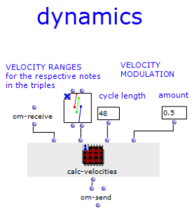
Dynamics
Different random ranges for “red”, “green” and “blue” notes can be defined for the volume or velocity. The values generated in this way can also be modulated sinusoidally so that, for example, the volume can rise and fall over longer periods of time. This requires the specification of a wavelength in the number of notes and the maximum deviation factor.
Accompaniment
PixelWaltz offers the option of generating an accompanying voice, which consists of individual additional tones in a desired fixed note number frequency. If this is not divisible by 3, a polymetric is often created. The pitch is determined randomly and can be between 3 and 6 semitones below the respective “accompanied” note.
Image processing
In order to create further variation, the sonification section of PixelWaltz is preceded by tools for manipulating the input image. In addition to adjusting the image size, brightness and contrast, it is also possible to shift the color values and thus recolor the image. The changes in the musical translation are immediately noticeable: More brightness leads to a higher average pitch, more contrast reduces the number of different pitch values. With a blue-dominated image, the last notes of the triplet will usually be the highest.
Sound results
The tonal results naturally differ depending on the input – but photographed material in particular often leads to the same wave-like overall structure, which winds irregularly and at a slow tempo chromatically, sometimes upwards, sometimes downwards. The accompaniment supports this effect and can form a counter-pulse to the main voice.
Abstract: A project on the use of random processes in a musical context. Basically, two different models are used. These generate chord sequences, which are then provided with a rhythm and an overlying melody.
Responsible: Moritz Reiser
Overview
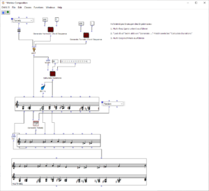
The overall structure of the program, which corresponds to the content of the main patch, can be seen in Figure 1. At the top is the selection of the algorithm to be used for chord progression generation. This can be selected via the selection field at the top left. The two input fields of the subpatches can be used to specify the desired length and the starting chord or the key of the composition.
This is followed by a random determination of the respective tone lengths. Here you can set the tempo in BPM as well as the frequencies of the tone lengths occurring in multiples of quarter notes. The respective start times of the chords are calculated from the calculated durations using a “dx→x” function. When using the program, care must be taken here that Open Music calculates new random numbers in both strings due to the output being used twice, as a result of which the relationship between the start time and the tone duration is lost. This can be remedied by locking the subpatches for chord progression and tone length generation with “Lock Eval” after running the program once and then running it again to adjust the start times to the now saved tone durations (see information panel in the main patch). The third major step in the overall process is the generation of a melody that lies above the chord sequence. Here, a note is selected from the underlying chord and shifted up an octave. You can set whether this should always be a random chord tone or whether the tone closest to or furthest away from the preceding melody tone should be selected.
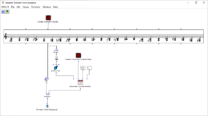
The result is then visualized at the bottom in a multi-seq object.
Figure 1: Overall structure of the composition process
Chord progression generation
Two algorithms are available for generating the chord sequence. The desired length of the sequence, which corresponds to the number of chords, and the starting chord or the key are transferred to them.
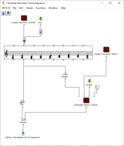
Harmonic chord sequence using Markov chain
The sequence of the first algorithm can be seen in Figure 2. The subpatch “Create Harmonic Chords” generates the basic set of chords that will be used in the following. This corresponds to the usual levels of counterpoint theory and, in addition to the tonic, subdominant, dominant and their parallels, contains a diminished chord on the seventh degree, a sixth ajoutée of the subdominant and a dominant seventh chord. The “Key” input adds a value corresponding to the desired key to these chords.
Figure 2: Subpatch for generating a harmonic chord sequence using a Markov chain
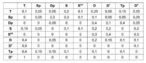
The “Create Transition Matrix” subpatch generates a matrix with transition probabilities for the individual chords. For each chord step, the probability with which it transitions to a certain other chord is determined. The probability values were chosen arbitrarily according to the usual processes in counterpoint theory and adjusted experimentally. For each chord it was investigated how likely it is to transition from this chord to another chord, so that the result corresponds to the conventions of counterpoint theory and allows a frequent return to the tonic level in order to focus on it. The exact transition probabilities are listed in the following table, whereby the initial sounds are listed in the left-hand column and the transitions are represented line by line.
Table 1. Transition probabilities of the harmonies of corresponding chord levels
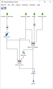
The generation of the chord sequence finally takes place in the patch “Generate Markov Series”, which is shown in Figure 3. This initially only works with the numbering of the chord steps, which is why it is sufficient to pass it the length of the chord list. The Lisp function “Markov Synthesis” now generates a chord sequence of the desired length using the transition matrix. As it is not guaranteed that the last chord in the sequence generated in this way corresponds to the tonic, another Lisp function is used, which generates further chords until the tonic is reached. As the steps have only been numbered so far, the chords valid for the respective steps are finally selected in order to obtain the finished chord sequence.
Figure 3: Subpatch for generating a chord sequence using Markov synthesis
Chromatic chord progression using a tone net
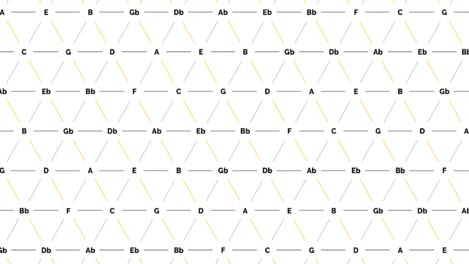
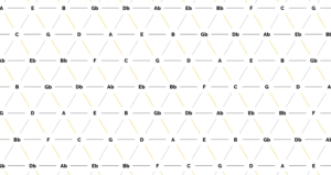
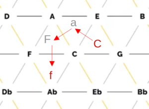
In contrast to the harmonic chord progression, all 24 major and minor chords of the chromatic scale are used here (see Figure 4). The special feature of this algorithm lies in the choice of transition probabilities. These are based on a so-called tone network, which is shown in Figure 5.
Figure 4: Subpatch for generating a chord sequence based on the tone net representation
Within the tone net, individual tones are applied and connected to each other. On the horizontal lines, the tones are each a fifth apart, while the diagonal lines show minor thirds (from top left to bottom right) and major thirds (from bottom left to top right). The resulting triangles each represent a triad, for example the triangle of the notes C, E and G results in the chord C major. All major and minor chords of the chromatic scale can be found. The Tonnetz representation is mostly used for analysis purposes, as a Tonnetz allows you to see directly how many tones two different triads share. One example is the analysis of classical music of the romantic and modern periods as well as film music, as the harmonic counterpoint rules used above are often neglected here in favor of chromatic and other previously unusual transitions. The distance between two chords in the tonal network can be a measure of whether the transition of one chord into the other is melodious or rather unusual. It is calculated from the number of edges that have to be crossed to get from one chord triangle to another. In other words, it corresponds to the degree of adjacency between two triangles, whereby a direct adjacency results from sharing an edge. Figure 6 shows an example of this: To get from the chord C major to the chord F minor, three edges have to be crossed, resulting in a distance of 3.
Figure 6: Example of determining the distance in the tone network using the transition from C major to F minor
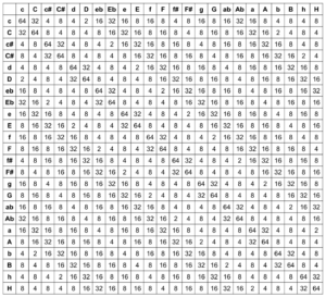
As part of the project, the transition probabilities are now calculated on the basis of the distances between chords in the tone network. It is only necessary to distinguish whether the active triad is a major or minor chord, as the same distances to other chords result for all keys within these two classes. This means that every transition can be calculated from C major or C minor and then shifted to the desired key by adding a value. Starting from both variants (C major and C minor), the distances to all other triads were first recorded in the tonal network:
Distances from C major:
Intervals from C minor:
In order to obtain probabilities from the intervals, all values were first subtracted from 6 to make larger intervals less probable. The results were then used as the exponent of the number 2 in order to give greater weighting to closer chords. Overall, this results in the formula
P=2^(6-x) ; P=probability, x=distance in the grid
to calculate the transition weights. These result in the following matrix for all possible chord combinations, from which 342 probabilities result when divided by the row sum.
Within the patch, the Lisp function “Generate Tonnetz Series” first determines whether the active chord is a major or minor triad. As with the harmonic procedure, only the numbers 0-23 are used initially, this can be determined using a simple modulo-2 calculation. Depending on the result, the respective probability vector is used, a new chord is determined and finally the previous step is added. If the result is a number greater than 23, 24 is subtracted in order to always remain within the same octave.
After the previously determined length of the sequence, this section is finished. There is no return to the tonic as in the previous section, as the chromaticism means that the tonic is not as pronounced as in the harmonic chord sequence.
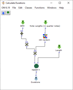
Determining the tone lengths
After a chord progression has been generated, random lengths are calculated for the individual triads. This is done in the “Calculate Durations” subpatch, which is shown in Figure 6. In addition to the desired BPM number, a list of note lengths is transferred as multiples of quarter notes. More probable values occur more frequently in this pool, so that a corresponding selection can be made via “nth-random”.
Figure 7: Subpatch for random determination of note durations
Melody generation
The basic melody generation process has already been described above: A tone is selected from the respective chord and transposed up an octave. This tone can be selected at random or according to the smallest or largest distance to the previous tone.
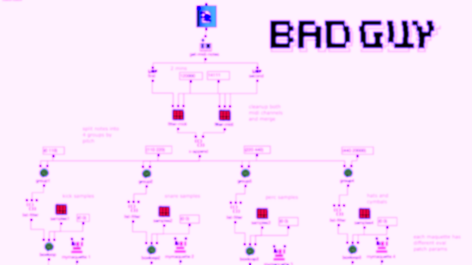
Inspired by the “Infinite Bad Guy” project, and all the very different versions of how some people have fueled their imaginations on that song, I thought maybe I could also experiment with creating a very loose, instrumental cover version of Billie Eilish’s “Bad Guy”.
Supervisor: Prof. Dr. Marlon Schumacher
A study by: Kaspars Jaudzems
Winter semester 2021/22
University of Music, Karlsruhe
To the study:
Originally, I wanted to work with 2 audio files, perform an FFT analysis on the original and “replace” its sound content with content from the second file, based only on the fundamental frequency. However, after doing some tests with a few files, I came to the conclusion that this kind of technique is not as accurate as I would like it to be. So I decided to use a MIDI file as a starting point instead.
Both the first and second versions of my piece only used 4 samples. The MIDI file has 2 channels, so 2 files were randomly selected for each note of each channel. The sample was then sped up or down to match the correct pitch interval and stretched in time to match the note length.
The second version of my piece added some additional stereo effects by pre-generating 20 random pannings for each file. With randomly applied comb filters and amplitude variations, a bit more reverb and human feel was created.
Acoustic study version 1
Acousmatic study version 2
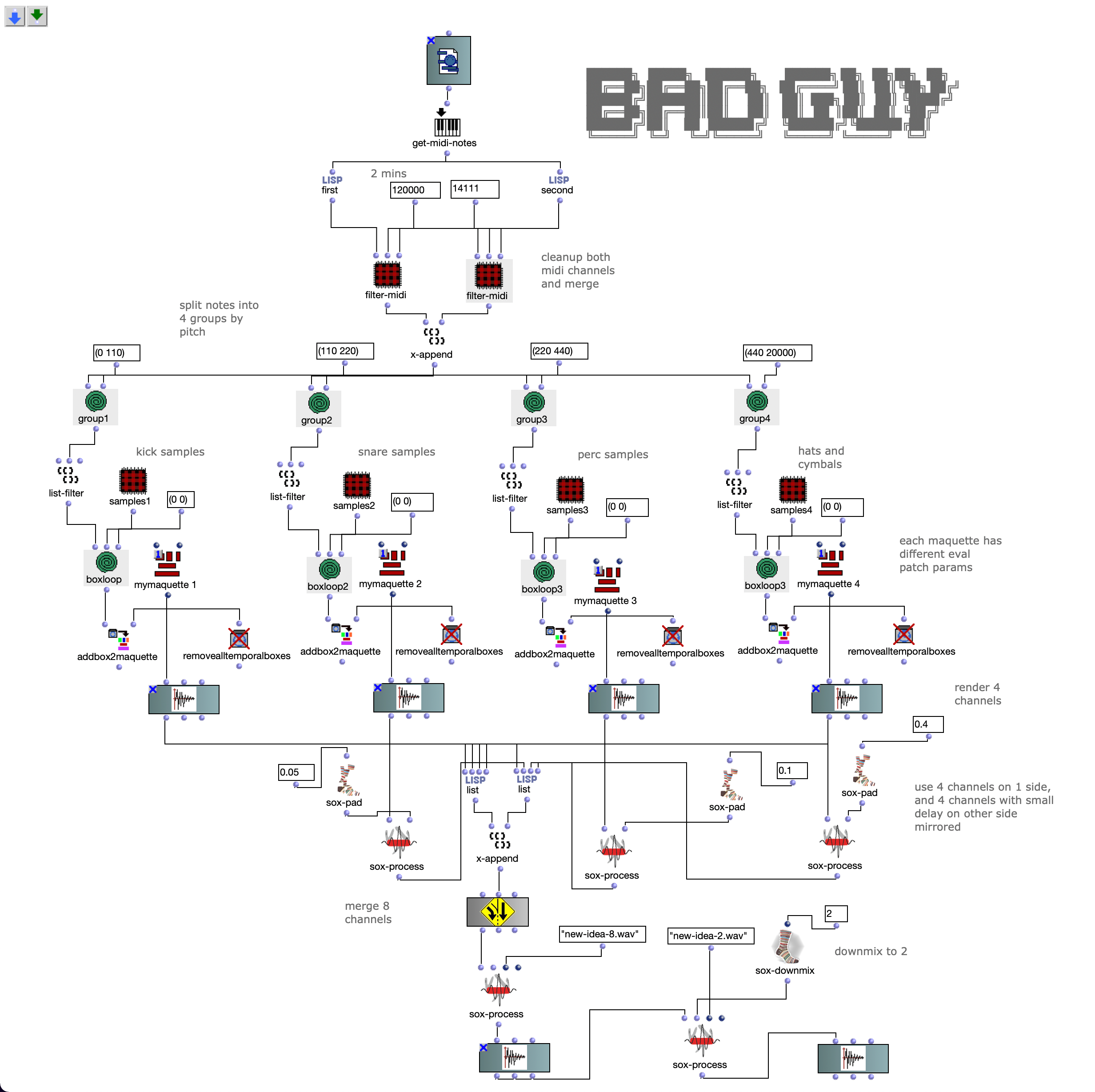
The third version was a much bigger change. Here the notes of both channels are first divided into 4 groups according to pitch. Each group covers approximately one octave in the MIDI file.
Then the first group (lowest notes) is mapped to 5 different kick samples, the second to 6 snares, the third to percussive sounds such as agogo, conga, clap and cowbell and the fourth group to cymbals and hats, using about 20 samples in total. A similar filter and effect chain is used here for stereo enhancement, with the difference that each channel is finely tuned. The 4 resulting audio files are then assigned to the 4 left audio channels, with the lower frequency channels sorted to the center and the higher frequency channels sorted to the sides. The same audio files are used for the other 4 channels, but additional delays are applied to add movement to the multi-channel experience.
Acousmatic study version 3
The 8-channel file was downmixed to 2 channels in 2 versions, one with the OM-SoX downmix function and the other with a Binauralix setup with 8 speakers.
Acousmatic study version 3 – Binauralix render
Extension of the acousmatic study – 3D 5th-order Ambisonics
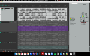
The idea with this extension was to create a 36-channel creative experience of the same piece, so the starting point was version 3, which only has 8 channels.
Starting point version 3
I wanted to do something simple, but also use the 3D speaker configuration in a creative way to further emphasize the energy and movement that the piece itself had already gained. Of course, the idea of using a signal as a source for modulating 3D movement or energy came to mind. But I had no idea how…
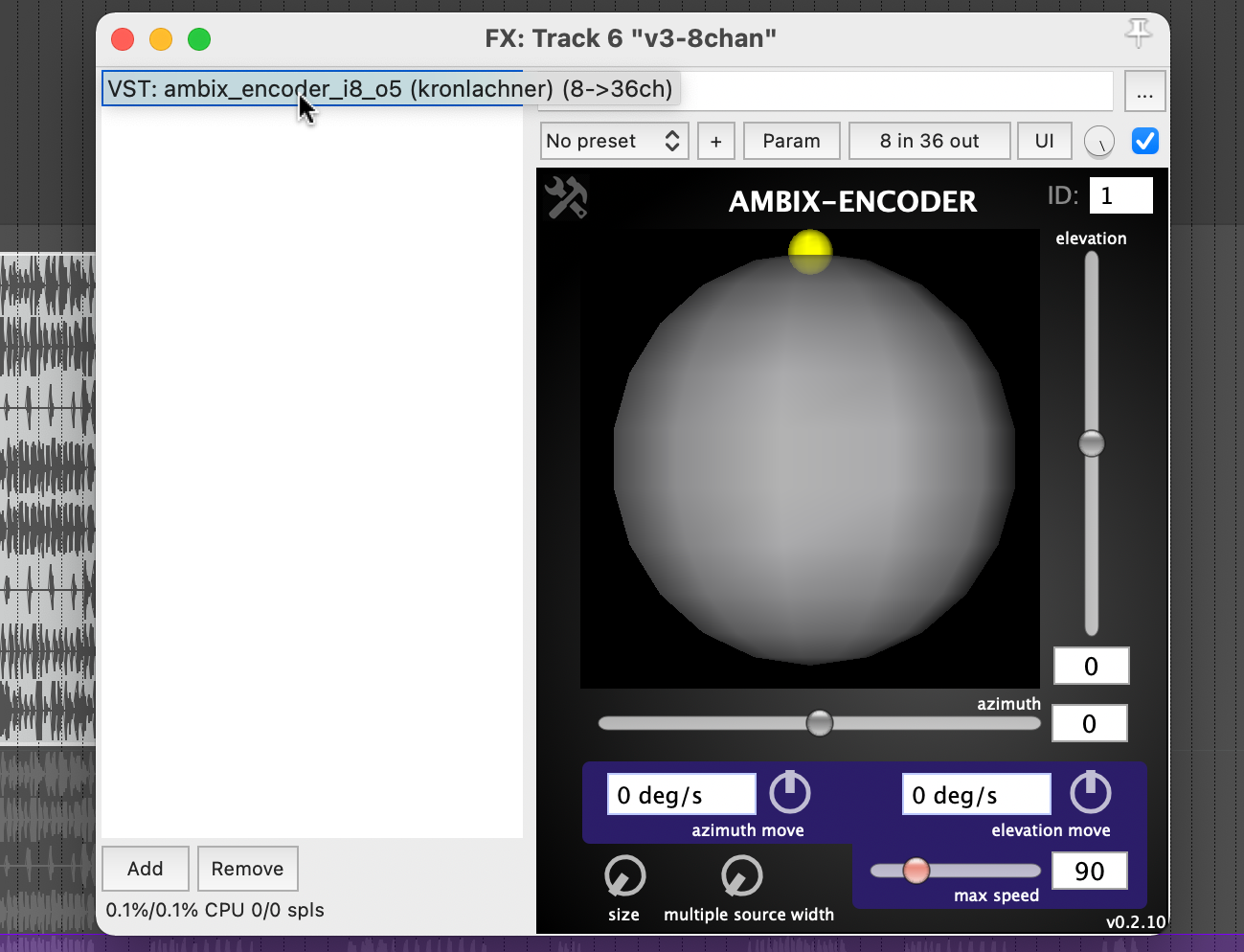
Plugin “ambix_encoder_i8_o5 (8 -> 36 chan)”
While researching the Ambix Ambisonic Plugin (VST) Suite, I came across the plugin “ambix_encoder_i8_o5 (8 -> 36 chan)”. This seemed to fit perfectly due to the matching number of input and output channels. In Ambisonics, space/motion is translated from 2 parameters: Azimuth and Elevation. Energy, on the other hand, can be translated into many parameters, but I found that it is best expressed with the Source Width parameter because it uses the 3D speaker configuration to actually “just” increase or decrease the energy.
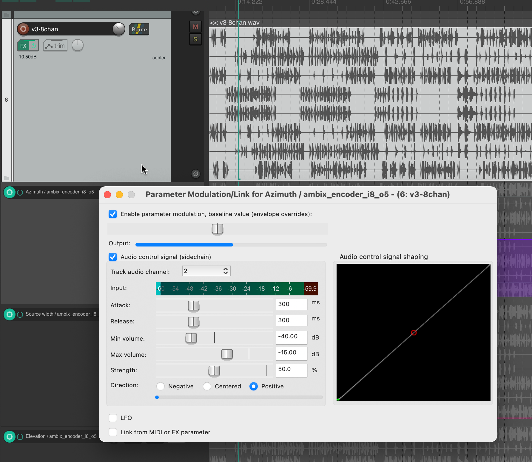
Knowing which parameters to modulate, I started experimenting with using different tracks as the source. To be honest, I was very happy that the plugin not only provided very interesting sound results, but also visual feedback in real time. When using both, I focused on having good visual feedback on what was going on in the audio piece as a whole.
This helped me to select channel 2 for Azimuth, channel 3 for Source Width and channel 4 for Elevation. If we trace these channels back to the original input midi file, we can see that channel 2 is assigned notes in the range of 110 to 220 Hz, channel 3 notes in the range of 220 to 440 Hz and channel 4 notes in the range of 440 to 20000 Hz. In my opinion, this type of separation worked very well, also because the sub-bass frequencies (e.g. kick) were not modulated and were not needed for this. This meant that the main rhythm of the piece could remain as a separate element without affecting the space or the energy modulations, and I think that somehow held the piece together.
Acousmatic study version 4 – 36 channels, 3D 5th-order Ambisonics – file was too big to upload
This article is about the three iterations of an acousmatic study by Zeno Lösch, which were carried out as part of the seminar “Symbolic Sound Processing and Analysis/Synthesis” with Prof. Dr. Marlon Schumacher at the HfM Karlsruhe. It deals with the basic conception, ideas, constructive iterations and the technical implementation with OpenMusic.
Responsible persons: Zeno Lösch, Master student Music Informatics at HfM Karlsruhe, 1st semester
Idea and concept
I got my inspiration for this study from the Freeze effect of GRM Tools.
This effect makes it possible to layer a sample and play it back at different speeds at the same time.
With this process you can create independent compositions, sound objects, sound structures and so on.
My idea is to program the same with Open Music.
For this I used the maquette and om-loops.
In the OpenMusicPatch you can find the different processes of layering the source material.
The source material is a “filtered” violin. This was created using the cross-synthesis process. This process of the source material was not created in Open Music.
Source material
Music cannot exist without time. Our perception connects the different sounds and seeks a connection. In this process, also comparable to rhythm, the individual object is connected to other objects. Digital sound manipulation makes it possible to use processes to create other sounds from one sound, which are related to the same sound.
For example, I present the sound in one form and change it at another point in the composition. This usually creates a connection, provided the listener can understand it.
You can change a transposition or the pitch in a similar way to notes.
This changes the frequency of a note. With digital material, this can lead to very exciting results. On a piano, the overtones of each note are related to the fundamental. These are fixed and cannot be changed with traditional sheet music.
With digital material, the effect that transposes plays a very important role. Depending on the type of effect, I have various possibilities to manipulate the material according to my own rules.
The disadvantage with instruments is that with a violin, for example, the player can only play the note once. Ten times the same note means ten violins.
In OpenMusic it is possible to play the “instrument” any number of times (as long as the computer’s processing power allows it).
Process
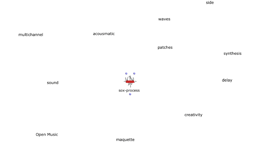
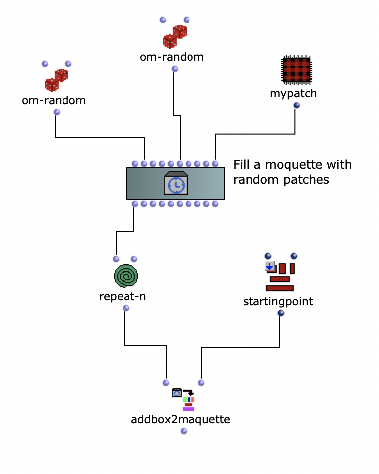
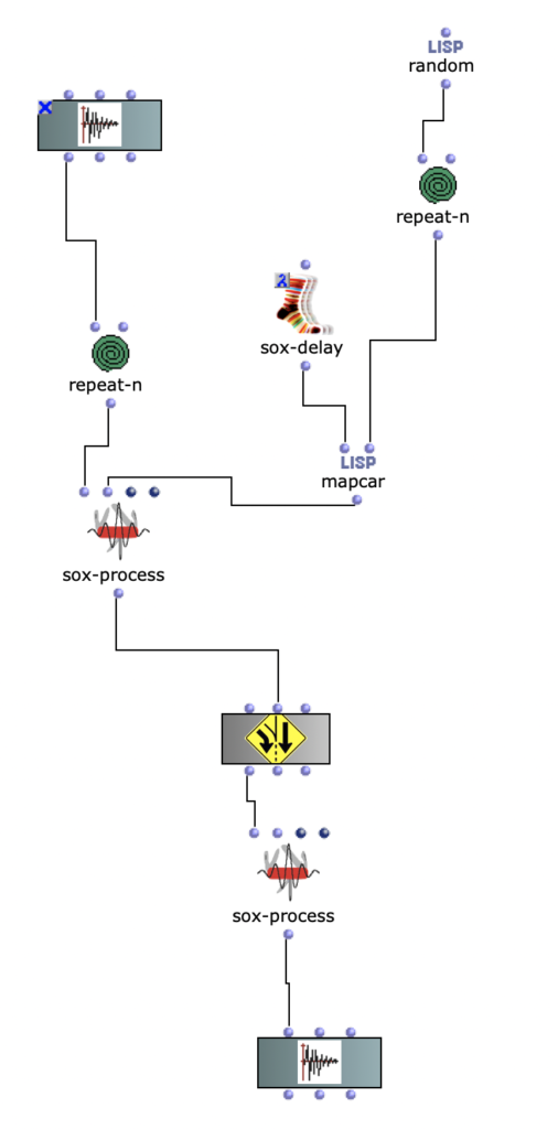
To recreate the Grm-Freeze, a moquette was first filled with empty patches.
Filling a moquette with empty patches
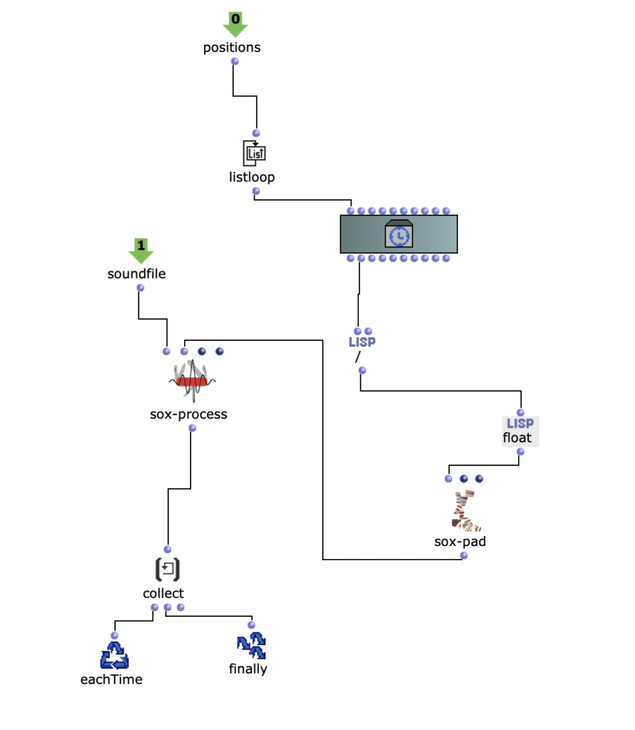
The soundfile was then rendered from the moquette with an om-loop to the positions of the empty patches.
Loop for soundfile positions
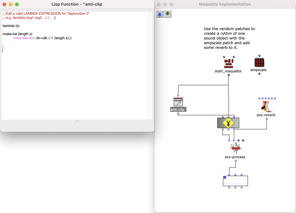
The following code was used to avoid clipping.
Sox-Mix and Anti Clip
Layer Study first iteration
The source material is presented at the beginning. In the course of the study, it is repeatedly changed and stacked in different ways.
The study itself also plays with the dynamics. Depending on the sound stacking algorithm, the dynamics in each sound object are changed. As there is more than one sound in time, these sounds are normalized depending on how many sounds are present in the algorithm to avoid clipping.
The study begins with the source material. This is then presented in a different temporal sequence.
This layer is then filtered and is also quieter. The next one develops into a “reverberant” sound. A continuum. The continuum remains it is presented differently again.
In the penultimate sound, a form of glissandi can be heard, which again ends in a sound that is similar to the second, but louder.
The process of stacking and changing the sound is very similar for each section.
The position is given by the empty patch in the moquette.
Then the y-position and x-position parameters are used for modulation
Implementation of the x and y positions as modulation parametersLayer study first iteration
Layer Study second iteration
I tried to create a different stereo image for each section.
Different rooms were simulated.
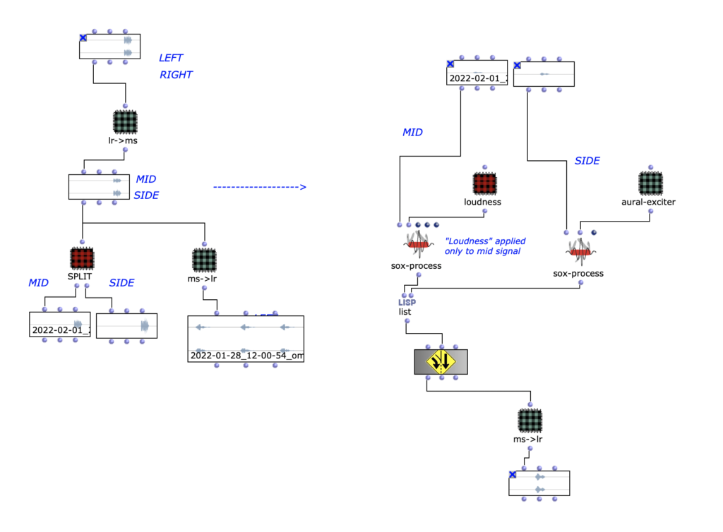
One technique that was used is the mid/side.
In this technique, the mid and side are extracted from a stereo signal using the following process:
Mid = (L R) * 0.5
Side = (L – R) * 0.5
An aural exciter has also been added.
In this process, the signal is filtered with a high-pass filter, distorted and added back to the input signal. This allows better definition to be achieved.
Through the mid/side, the aural exciter is only applied to one of the two and it is perceived as more “defined”.
To return the process to a stereo signal, the following process is used:
L = Mid Side
R = Mid – Side
Mid Side process
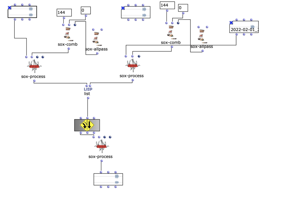
To further spatialize the sound, an all-pass filter and a comb filter were used to change the phase of the mid or side component.
Decorrelation of the phase
Layer Study Stereo
Layer Study third iteration
In this iteration, the stereo file was divided into eight speakers.
The different sections of the stereo composition were extracted and different splitting techniques were used.
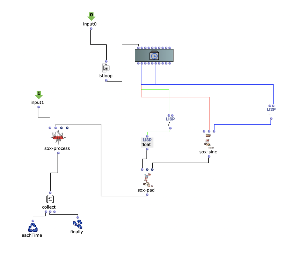
In one of these, a different fade in and fade out was used for each channel.
In an acousmatic version of a composition, this fade in and fade out can be achieved with the controls of a mixer.
A mapcar and repeat-n were used for this purpose.
Random fades for multichannel
The position of the respective channels was changed in the other processes. A delay was used.
A link to download the applications can be found at the end of this blogpost. This project was also presented as a paper at the 2022 International Conference on Technologies for Music Notation and Representation (TENOR 2022).
Modularity in Sound Synthesis Tools
This blogpost walks through the structure and usage of two applications of machine learning (ML) methods for sound notation and synthesis. The first application is a modular sample replacement engine that uses a supervised classification algorithm to segment and transcribe a drum beat, and then reconstruct that same drum beat with different samples. The second application is a texture synthesis engine that uses an unsupervised clustering algorithm to analyze and sort large numbers of audio files.
The applications were developed in OpenMusic using the OM-SoX modular synthesis/analysis framework. This was so that the applications could be as modular as possible. Modular, meaning that they could be customized, extended, and integrated into a user’s own OpenMusic workflow. We believe this modularity offers something new to the community of ML and sound synthesis/analysis tools currently available. The approach to sound synthesis and analysis used here involves reading and querying many separate audio files. Such an approach can be encompassed by the larger term of “corpus-based concatenative synthesis/analysis,” for which there are already several effective tools: the Caterpillar System, Audioguide, and OM-Pursuit. Additionally, OM-AI, ml.*, and zsa.descriptors are existing toolkits that integrate ML methods into Computer-Aided Composition (CAC) environments. While these tools are very precise, the internal workings of them are not immediately clear. By seeking for our applications to be modular, we mean that they can be edited, extended and integrated into existing CAC programs. It also means that they can be opened and up, examined, and reverse-engineered for a user’s own education.
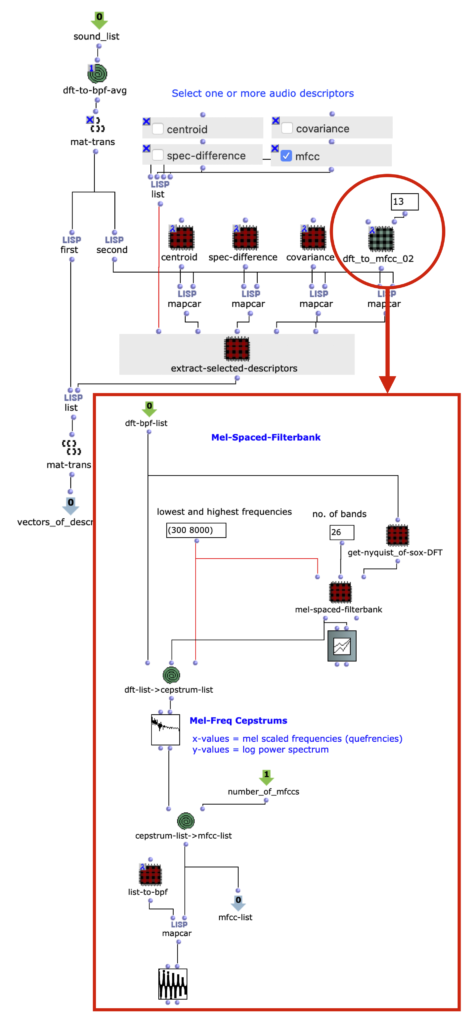
One example of this is in figure 1, our audio analysis engine. Audio descriptors are implemented as subpatches in lambda mode, and can be selected as needed for the input audio.
Figure 1: Interchangeable audio descriptors are set as patches in lambda mode. Here, a patch extracting 13 MFCCs is being used.
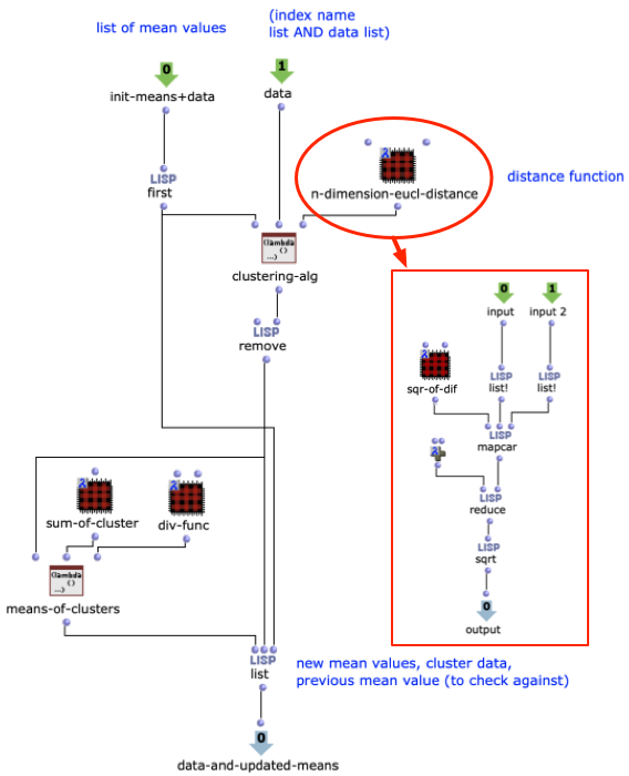
Another example is in figure 2, a customizable distance function in our texture synthesis application. This is the ML clustering algorithm that drives the application. Being a patch built from smaller OpenMusic objects, it is not only a tool for visualizing the algorithm at work, it also allows a user to edit it. For example, the n-dimension euclidean distance function could be substituted with another distance function, if needed.
Figure 2: A simple k-means clustering algorithm, built within an OpenMusic abstraction. The distance function takes the form of a subpatcher in lambda mode.
With the modularity of the project introduced, we will on the next page move on to the two specific applications.