Abstract: The entry describes the spatialization of the piece “Ode An Die Reparatur” (“Ode To The Repair”) (2021) and its transformation into a Higher Order Ambisonics version. A binaural mix of the finished piece makes it possible to understand the working process based on the result.
Supervisor: Prof. Dr. Marlon Schumacher
A contribution by: Jakob Schreiber
Piece
The piece “Ode An Die Reparatur” (2021) consists of four movements, each of which refers to a different aspect of a fictional machine. What was interesting about this process was to investigate the transition from machine sounds to musical sounds and to shape it over the course of the piece.
Production
The production resources for the piece were, on the one hand, a UHER tape recorder, which enables simple repitch changes and was predestined for the realization of this piece based on mechanical machines due to its functionality with motors and belts. SuperCollider was also used as a digital sound synthesis and alienation environment.
Structure
The piece consists of four movements.
First movement
The sound material of the beginning is composed of various recordings from a tape recorder, over which clearly audible, synthesized engine sounds are played alongside silence.
Second movement
The sound objects, some of which are reminiscent of birdsong, suddenly emerge from sterile silence into the foreground.
Third movement
The perforative characteristics inside a gearwheel are transformed into tonal resonances in the course of the movement.
Fourth movement
In the last movement, the engines play a monumental final hymn.
Spatialization
Based on the compositional form of the piece, the spatialization drafts adhere to the division into movements.
Working practice
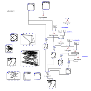
The working process can be divided into different sections, similar to the OM patch. In the laboratory section, I explored different forms of spatialization in terms of their aesthetic effect and examined their conformity with the compositional form of the existing piece.
In order to determine different trajectories, or fixed positions of sound objects, the visual assessment of the respective trajectories played an important role in addition to the auditory effect.
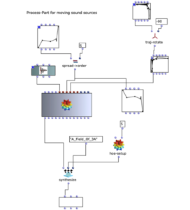
Ultimately, the parameters of the pre-selected trajectories were supplemented with a scattering curve, finely adjusted and finally transformed into a fifth-order Higher Order Ambisonics audio file via a chain of modules.
Iteratively, the synthesized multi-channel files are added to the overall structure in REAPER and their effect is examined before they are run through the synthesis process again with an optimized set of parameters and trajectories.
More details on the individual sentences
First, you can listen to the binaural version of the spatialized piece as a whole. The approaches of the individual parts are described briefly below
In the first part, the long, drawn-out clouds of sound, lying on top of each other like layers, move according to the basic tempo of the movement. The trajectories lie in a U-shape around the listening area, covering only the sides and front.
Second movement
Individual sound objects should be heard from very different positions. Almost percussive sounds from all directions of the room make the listener’s attention jump.
Third movement
The sonic material of this part is a sound synthesis based on the sound of cogwheels or gears. The focus here was on immersion in the fictitious machine. From this very sound material, resonances and other changes create horizontal tones that are strung together to form short motifs.
The spatialization concept for this part is made up of moving and partly static objects. The moving ones create an impression of spatial immersion at the beginning of the movement. At the end of the movement, two relatively static objects are added to the left and right of the stereo base, which primarily emphasize the melodic aspects of the sound and merely oscillate fleetingly on the vertical axis at their respective positions.
Fourth movement
The instrumentation of this part of the piece consists of three simulations of an electric motor, each of which follows its own voice. In order to separate the individual voices a little better, I decided to treat each of the four motors as an individual sound object. To support the monumental character of the final part, the objects only move very slowly through the fictitious space.
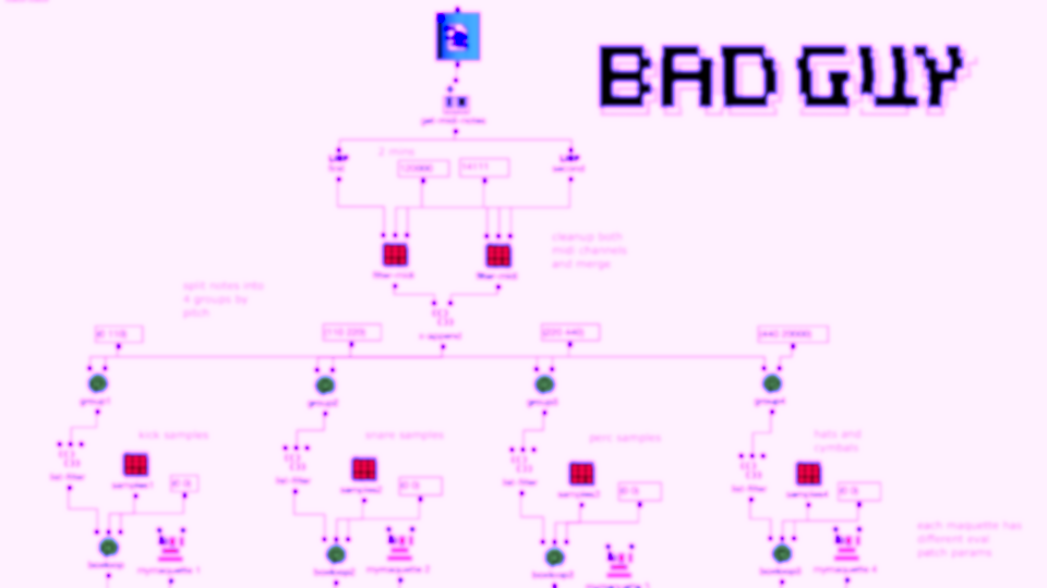
Inspired by the “Infinite Bad Guy” project, and all the very different versions of how some people have fueled their imaginations on that song, I thought maybe I could also experiment with creating a very loose, instrumental cover version of Billie Eilish’s “Bad Guy”.
Supervisor: Prof. Dr. Marlon Schumacher
A study by: Kaspars Jaudzems
Winter semester 2021/22
University of Music, Karlsruhe
To the study:
Originally, I wanted to work with 2 audio files, perform an FFT analysis on the original and “replace” its sound content with content from the second file, based only on the fundamental frequency. However, after doing some tests with a few files, I came to the conclusion that this kind of technique is not as accurate as I would like it to be. So I decided to use a MIDI file as a starting point instead.
Both the first and second versions of my piece only used 4 samples. The MIDI file has 2 channels, so 2 files were randomly selected for each note of each channel. The sample was then sped up or down to match the correct pitch interval and stretched in time to match the note length.
The second version of my piece added some additional stereo effects by pre-generating 20 random pannings for each file. With randomly applied comb filters and amplitude variations, a bit more reverb and human feel was created.
Acoustic study version 1
Acousmatic study version 2
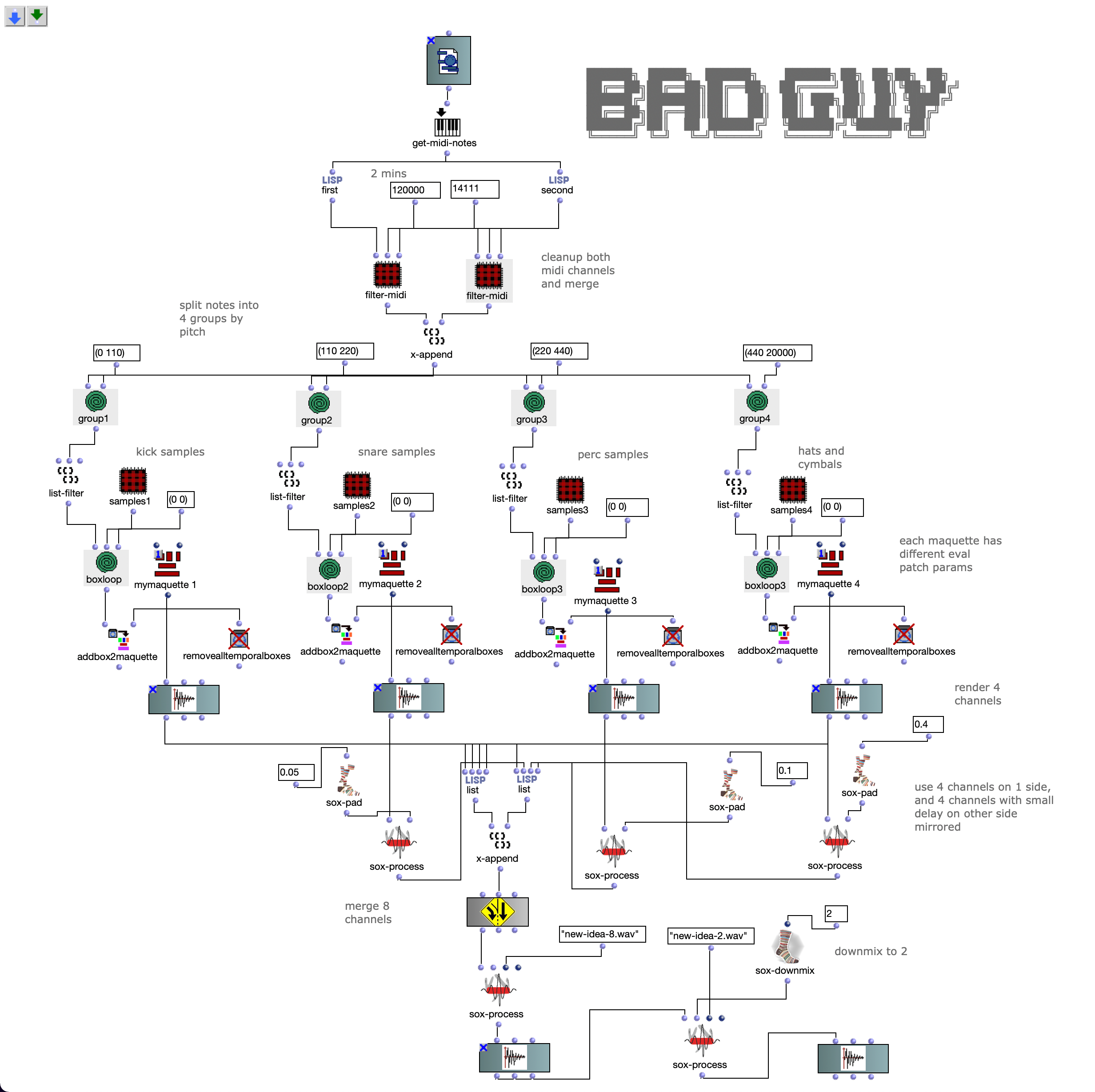
The third version was a much bigger change. Here the notes of both channels are first divided into 4 groups according to pitch. Each group covers approximately one octave in the MIDI file.
Then the first group (lowest notes) is mapped to 5 different kick samples, the second to 6 snares, the third to percussive sounds such as agogo, conga, clap and cowbell and the fourth group to cymbals and hats, using about 20 samples in total. A similar filter and effect chain is used here for stereo enhancement, with the difference that each channel is finely tuned. The 4 resulting audio files are then assigned to the 4 left audio channels, with the lower frequency channels sorted to the center and the higher frequency channels sorted to the sides. The same audio files are used for the other 4 channels, but additional delays are applied to add movement to the multi-channel experience.
Acousmatic study version 3
The 8-channel file was downmixed to 2 channels in 2 versions, one with the OM-SoX downmix function and the other with a Binauralix setup with 8 speakers.
Acousmatic study version 3 – Binauralix render
Extension of the acousmatic study – 3D 5th-order Ambisonics
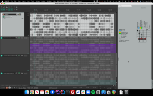
The idea with this extension was to create a 36-channel creative experience of the same piece, so the starting point was version 3, which only has 8 channels.
Starting point version 3
I wanted to do something simple, but also use the 3D speaker configuration in a creative way to further emphasize the energy and movement that the piece itself had already gained. Of course, the idea of using a signal as a source for modulating 3D movement or energy came to mind. But I had no idea how…
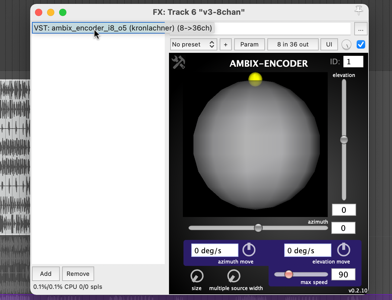
Plugin “ambix_encoder_i8_o5 (8 -> 36 chan)”
While researching the Ambix Ambisonic Plugin (VST) Suite, I came across the plugin “ambix_encoder_i8_o5 (8 -> 36 chan)”. This seemed to fit perfectly due to the matching number of input and output channels. In Ambisonics, space/motion is translated from 2 parameters: Azimuth and Elevation. Energy, on the other hand, can be translated into many parameters, but I found that it is best expressed with the Source Width parameter because it uses the 3D speaker configuration to actually “just” increase or decrease the energy.
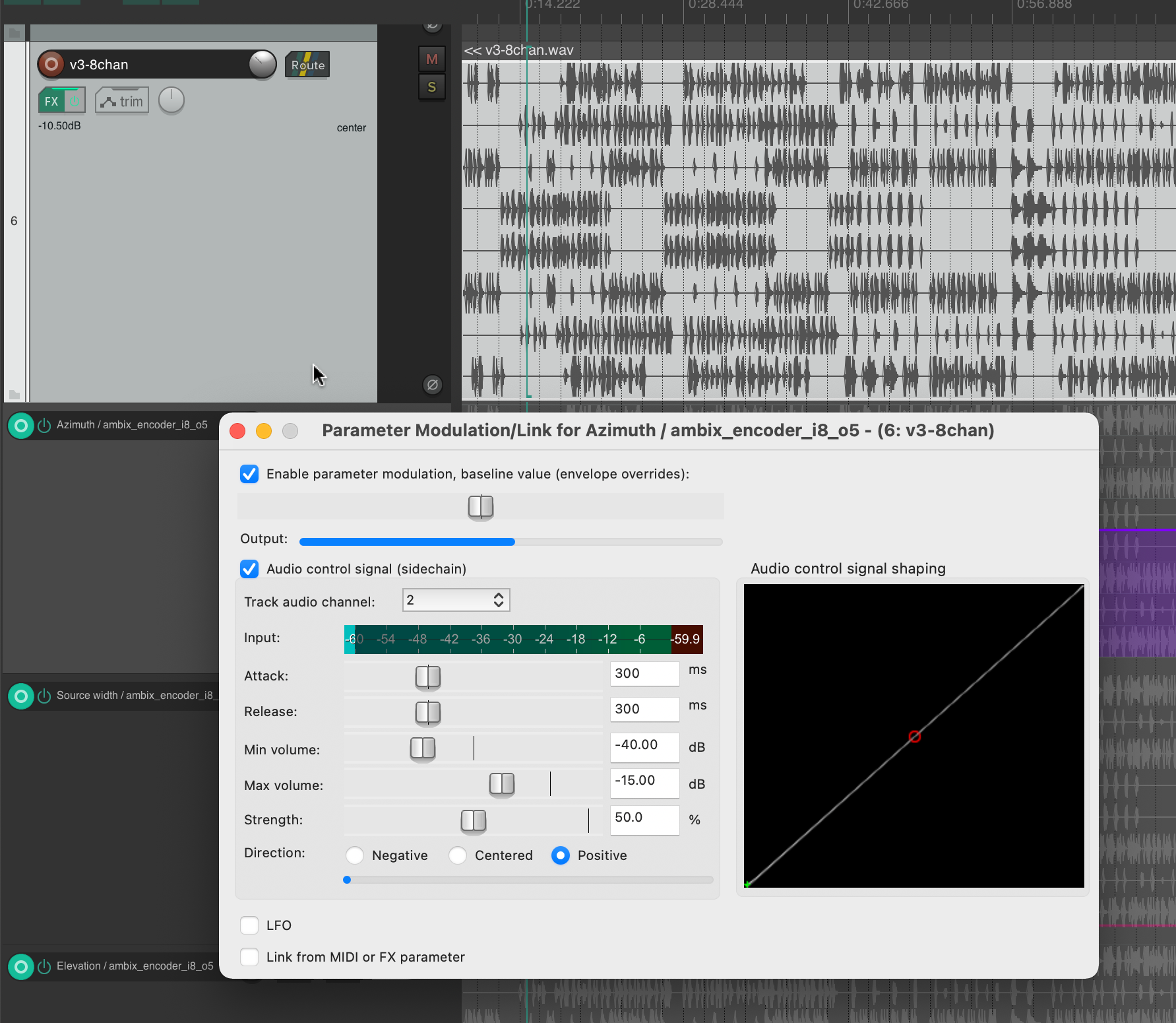
Knowing which parameters to modulate, I started experimenting with using different tracks as the source. To be honest, I was very happy that the plugin not only provided very interesting sound results, but also visual feedback in real time. When using both, I focused on having good visual feedback on what was going on in the audio piece as a whole.
This helped me to select channel 2 for Azimuth, channel 3 for Source Width and channel 4 for Elevation. If we trace these channels back to the original input midi file, we can see that channel 2 is assigned notes in the range of 110 to 220 Hz, channel 3 notes in the range of 220 to 440 Hz and channel 4 notes in the range of 440 to 20000 Hz. In my opinion, this type of separation worked very well, also because the sub-bass frequencies (e.g. kick) were not modulated and were not needed for this. This meant that the main rhythm of the piece could remain as a separate element without affecting the space or the energy modulations, and I think that somehow held the piece together.
Acousmatic study version 4 – 36 channels, 3D 5th-order Ambisonics – file was too big to upload
Abstract: Spectral Select explores the spectral content of one sample and the amplitude curve of a second sample and unites them in a new musical context. The meditative character of the output created by iteration is both contrasted and structured by louder amplitude peaks. In a revised version, Spectral Select was spatialized in Ambisonics HOA-5 format.
Supervisor: Prof. Dr. Marlon Schumacher
A study by: Anselm Weber
Winter semester 2021/22 University of Music, Karlsruhe
About the study: In which forms of expression is the connection between frequency and amplitude expressed ? Are both areas intrinsically connected and if so, what could be approaches to redesigning this order? Such questions have occupied me for some time. That’s why the attempt to redesign them is the core topic of Spectral Select. I was inspired by AudioSculpt from IRCAM, which we got to know in our course: “Symbolic Sound Processing and Analysis/Synthesis” together with Prof. Dr. Marlon Schumacher and Brandon L. Snyder and which we partially rebuilt.
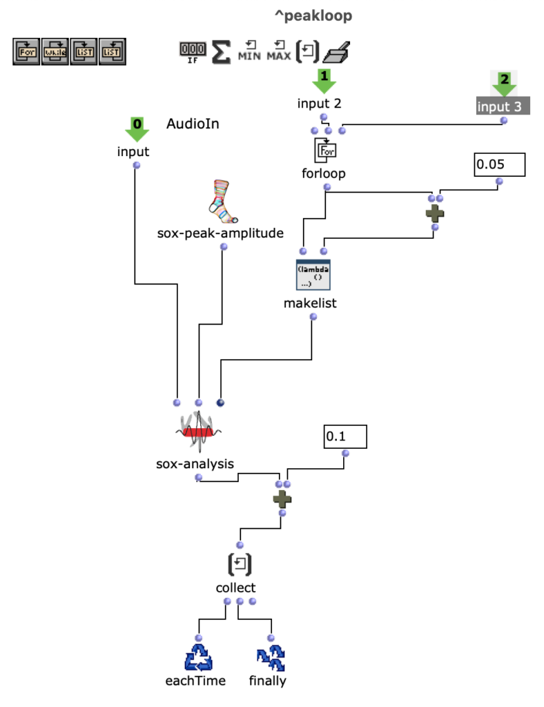
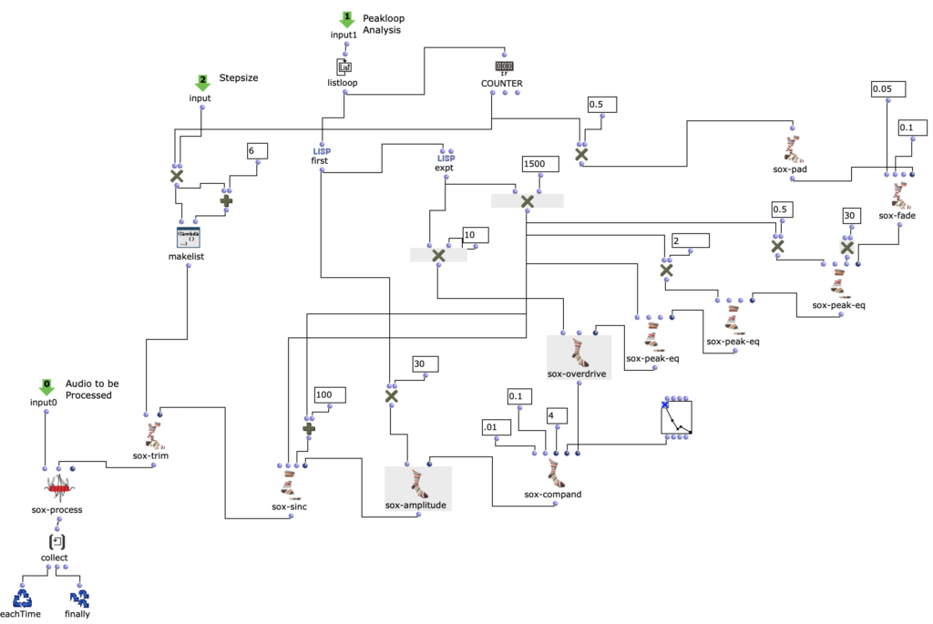
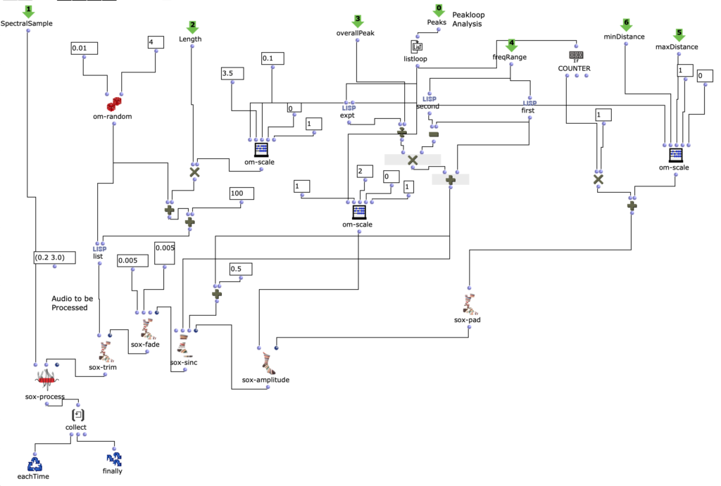
Spectral Edit works on a similar principle, but instead of having a user work out interesting areas within a spectrum of a sample, it was decided to use a second audio sample. This additional sample (from now on referred to as “amplitude sound” in the course of this article) determines how the first sample (from now on referred to as “spectral sound”) is to be processed by OM-Sox. To achieve this, two loops are used: First, individual amplitude peaks are analyzed out of the amplitude sound in the first “peakloop”. This analysis is then used in the heart of the patch, the “choosefreq” loop, to select interesting sub-ranges from the spectral sample. Loud peaks filter narrower bands from higher frequency ranges and form a contrast to weaker peaks, which filter somewhat broader bands from lower frequency ranges.
peakloop – Analysis
choosefreq Loop – Audio Processing
How small the respective iteration steps are affects both the length and the resolution of the overall output. Depending on the sample material, a large number of short grains or fewer but longer subsections can be created. However, both of these parameters can be selected freely and independently of each other.
In the enclosed piece, for example, a relatively high resolution (i.e. an increased number of iteration steps) was chosen in combination with a longer duration of the cut sample. This creates a rather meditative character, whereby no two sections will be 100% identical, as there are constantly minimal changes under the peak amplitudes of the amplitude sound. The still relatively raw result of this algorithm is the first version of my acousmatic study.
Acousmatic study version 1
The subsequent revision step was primarily aimed at working out the differences between the individual iteration steps more precisely. For this purpose, a series of effects were used, which in turn behave differently depending on the peak amplitude of the amplitude sound. To make this possible, the series of effects was integrated directly into the peak loop.
Acousmatic study version 2
In the third and final revision step, the audio was spatialized to 8 channels. The individual channels sound into each other and change their position in a clockwise direction. This means that the basic character of the piece remains the same, but it is now also possible to follow the “working through” of the choosefreq loop spatially. To maintain this spatiality, the output was then converted to binaural stereo for the upload using Binauralix.
Acoustic study version 3 – Binaural
Spectral Select – Ambisonics
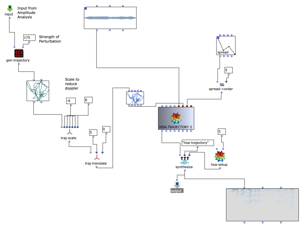
In the course of a further revision, Spectral Select was re-spatialized using the spatialization class “Hoa-Trajectory” from OM-Prisma and converted to the Ambisonics format. To ensure that this step fits in well conceptually and sonically with the previous edits, the amplitude sound should also play an important role in the spatial position. The possibilities for spatializing sounds with the help of Open Music and OM Prism are numerous. In the end, it was decided to work with Hoa-Trajectory. Here, the sound source is not bound to a fixed position in space and can be described with a trajectory that is scaled to the total duration of the audio input.
Spatialization with HOA.TRAEJECTORY
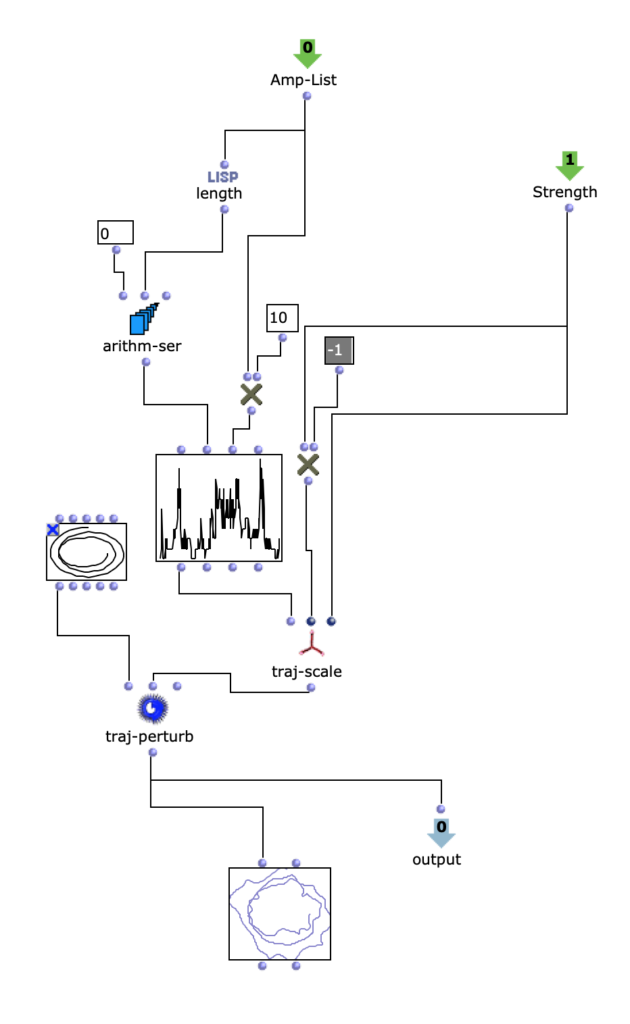
The trajectory is created depending on the amplitude analysis in the previous step. A simple, three-dimensional circular movement, which spirals downwards, is perturbed with a more complex, two-dimensional curve. The Y-values of the more complex curve correspond to the analyzed amplitude values of the amplitude sound. Depending on the scaling of the amplitude curve, this results in more or less pronounced deviations in the circular motion. Higher amplitude values therefore ensure more extensive movements in space.
It is interesting to note that OM-Prisma also takes Doppler effects into account. As a result, it is also audible that at higher amplitude values, more extreme distances to the listening position are covered in the same time. This step therefore has a direct influence on the timbre of the entire piece. Depending on the scaling of the trajectory, fast movements can be strongly overemphasized, but artifacts can also occur (if the distance is too great). To get a better impression, 2 different runs of the algorithm with different distances to the listener follow.
Version with extreme Doppler effects which can result in artifacts – binaural stereo
Versionwith closer distance and more moderate Dopp ler effects – Binaural Stereo
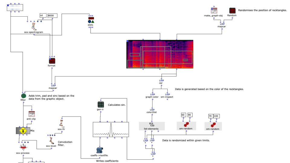
In contrast to the previous sound examples, the spectral sound and amplitude sound have been replaced in this example. This is a longer sound file for analyzing the amplitudes and a less distorted drone as a spectral sound. The idea behind this project is to experiment with different sound files anyway. Therefore, the old algorithm has been reworked to offer more flexibility with different sound files:
Revised scalable version of the old algorithm for selecting from the spectral sound
In addition, a randomized selection is now made from the spectral sound on the time axis. As a result, any shaping context should come from the magnitude of the amplitude sound and any timbre should be extracted from the spectral sound.
In this article I present my ideas, creative processes and technical data for the patch programmed for the class “Symbolic Sound Processing and Analysis/Synthesis” with Prof. Marlon Schumacher. The idea of this text is to show the technical solutions for my creative ideas and to share the knowledge gained to help the reader with their ideas. The purpose of this patch is to take sounds from everyday life and transform them into your own composition using several processes within Open Music.
The initial idea of the piece was to transform everyday sounds, for example the sound of a kettle, into a different, processed sound by implementing technical solutions in Open Music. This patch processes and merges several files into one composition. There are three iterations of the patch that I worked on during the semester. I will describe them in chronological order.
The original idea for the patch came from musique concréte. I wanted to make a 2-minute piece from concrete sounds (not synthesized in Open Music, but recorded). This patch consists of three subpatches that are connected to the maquette in the main patch.
This article is about the three iterations of an acousmatic study by Zeno Lösch, which were carried out as part of the seminar “Symbolic Sound Processing and Analysis/Synthesis” with Prof. Dr. Marlon Schumacher at the HfM Karlsruhe. It deals with the basic conception, ideas, constructive iterations and the technical implementation with OpenMusic.
Responsible persons: Zeno Lösch, Master student Music Informatics at HfM Karlsruhe, 1st semester
Idea and concept
I got my inspiration for this study from the Freeze effect of GRM Tools.
This effect makes it possible to layer a sample and play it back at different speeds at the same time.
With this process you can create independent compositions, sound objects, sound structures and so on.
My idea is to program the same with Open Music.
For this I used the maquette and om-loops.
In the OpenMusicPatch you can find the different processes of layering the source material.
The source material is a “filtered” violin. This was created using the cross-synthesis process. This process of the source material was not created in Open Music.
Source material
Music cannot exist without time. Our perception connects the different sounds and seeks a connection. In this process, also comparable to rhythm, the individual object is connected to other objects. Digital sound manipulation makes it possible to use processes to create other sounds from one sound, which are related to the same sound.
For example, I present the sound in one form and change it at another point in the composition. This usually creates a connection, provided the listener can understand it.
You can change a transposition or the pitch in a similar way to notes.
This changes the frequency of a note. With digital material, this can lead to very exciting results. On a piano, the overtones of each note are related to the fundamental. These are fixed and cannot be changed with traditional sheet music.
With digital material, the effect that transposes plays a very important role. Depending on the type of effect, I have various possibilities to manipulate the material according to my own rules.
The disadvantage with instruments is that with a violin, for example, the player can only play the note once. Ten times the same note means ten violins.
In OpenMusic it is possible to play the “instrument” any number of times (as long as the computer’s processing power allows it).
Process
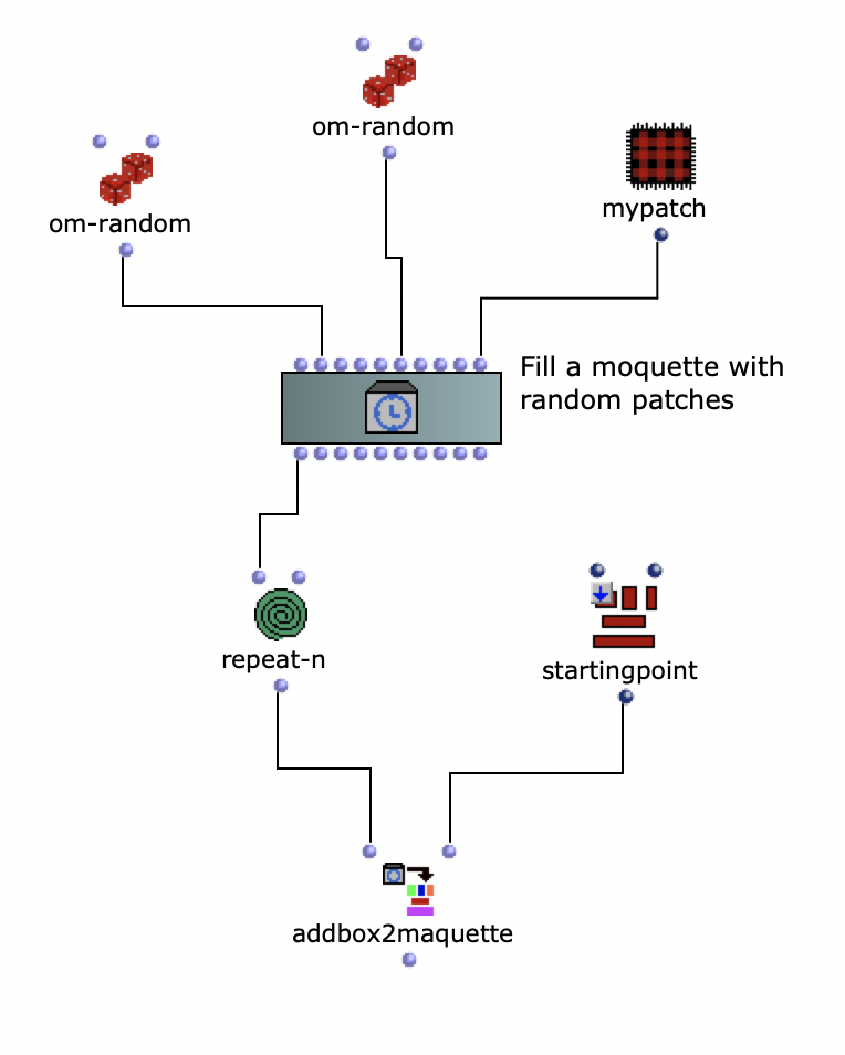
To recreate the Grm-Freeze, a moquette was first filled with empty patches.
Filling a moquette with empty patches
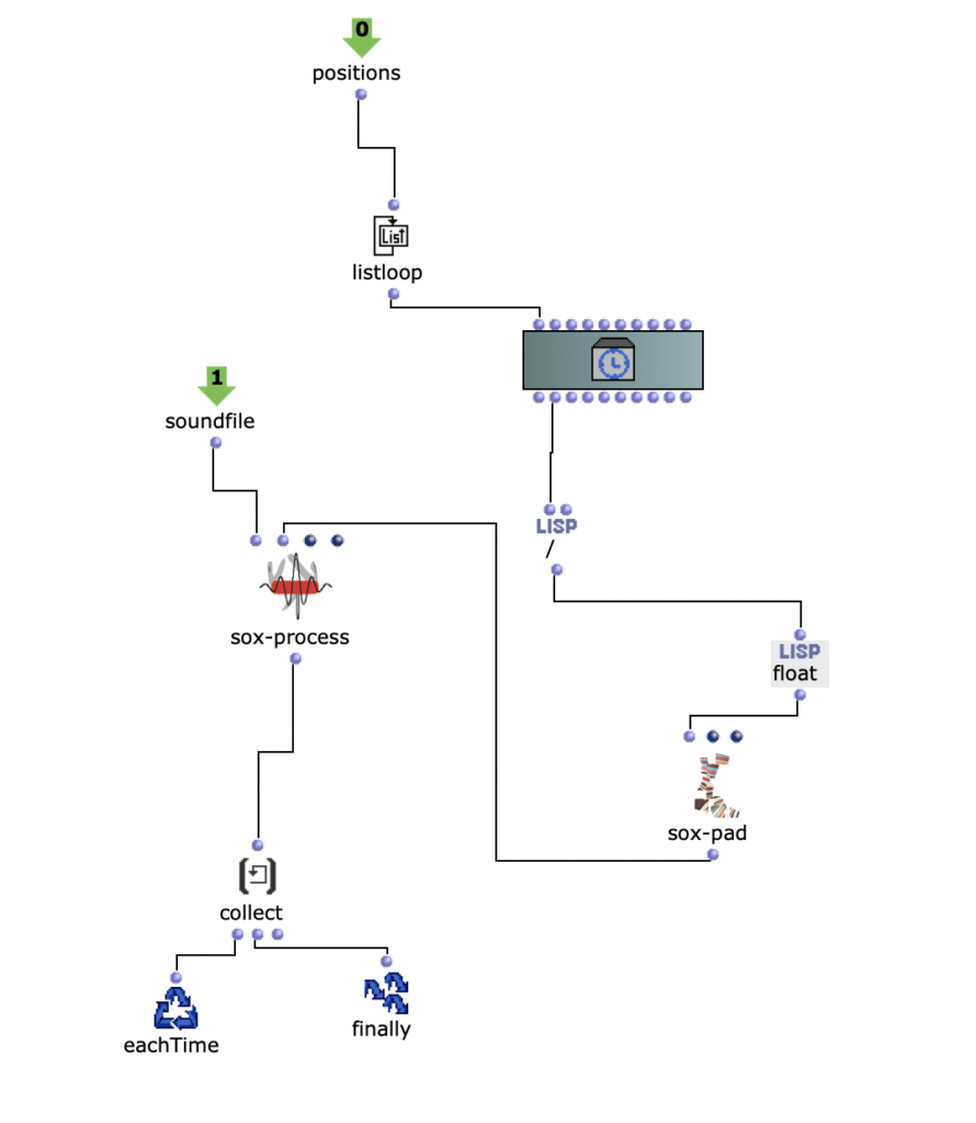
The soundfile was then rendered from the moquette with an om-loop to the positions of the empty patches.
Loop for soundfile positions
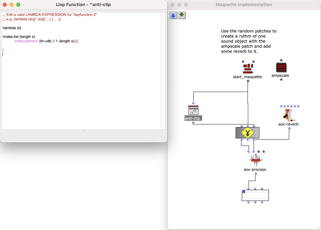
The following code was used to avoid clipping.
Sox-Mix and Anti Clip
Layer Study first iteration
The source material is presented at the beginning. In the course of the study, it is repeatedly changed and stacked in different ways.
The study itself also plays with the dynamics. Depending on the sound stacking algorithm, the dynamics in each sound object are changed. As there is more than one sound in time, these sounds are normalized depending on how many sounds are present in the algorithm to avoid clipping.
The study begins with the source material. This is then presented in a different temporal sequence.
This layer is then filtered and is also quieter. The next one develops into a “reverberant” sound. A continuum. The continuum remains it is presented differently again.
In the penultimate sound, a form of glissandi can be heard, which again ends in a sound that is similar to the second, but louder.
The process of stacking and changing the sound is very similar for each section.
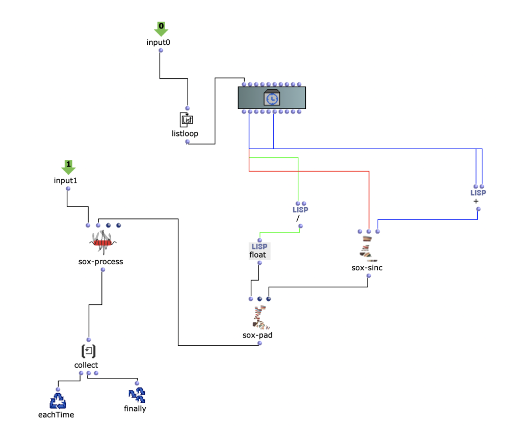
The position is given by the empty patch in the moquette.
Then the y-position and x-position parameters are used for modulation
Implementation of the x and y positions as modulation parametersLayer study first iteration
Layer Study second iteration
I tried to create a different stereo image for each section.
Different rooms were simulated.
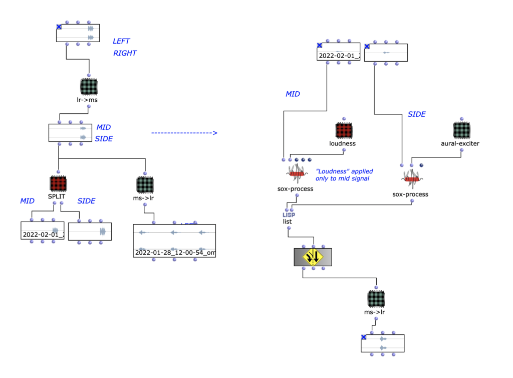
One technique that was used is the mid/side.
In this technique, the mid and side are extracted from a stereo signal using the following process:
Mid = (L R) * 0.5
Side = (L – R) * 0.5
An aural exciter has also been added.
In this process, the signal is filtered with a high-pass filter, distorted and added back to the input signal. This allows better definition to be achieved.
Through the mid/side, the aural exciter is only applied to one of the two and it is perceived as more “defined”.
To return the process to a stereo signal, the following process is used:
L = Mid Side
R = Mid – Side
Mid Side process
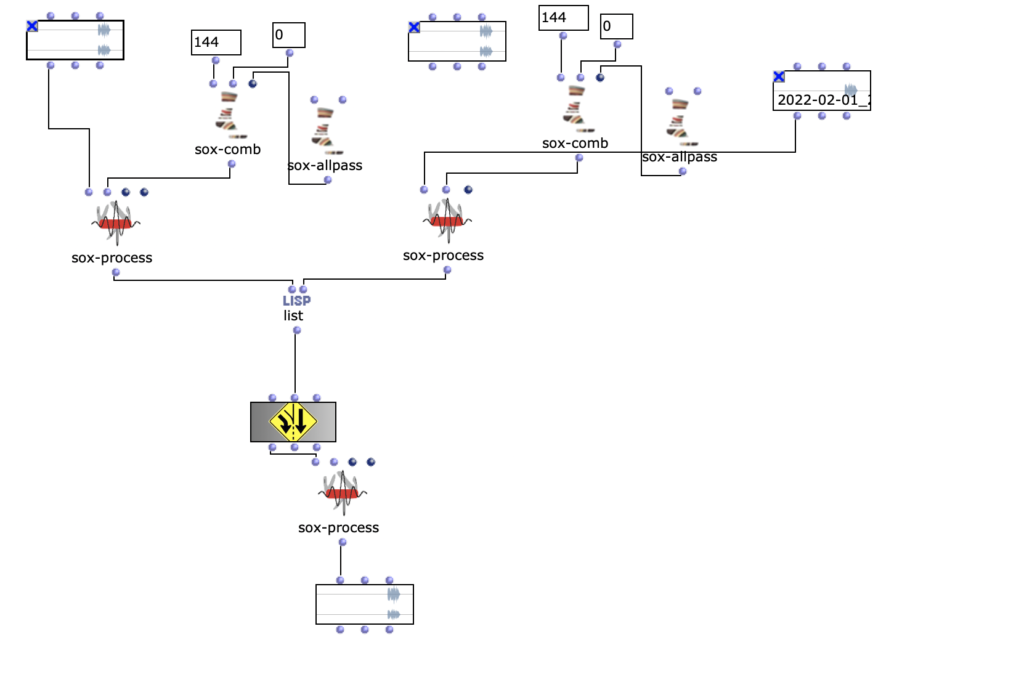
To further spatialize the sound, an all-pass filter and a comb filter were used to change the phase of the mid or side component.
Decorrelation of the phase
Layer Study Stereo
Layer Study third iteration
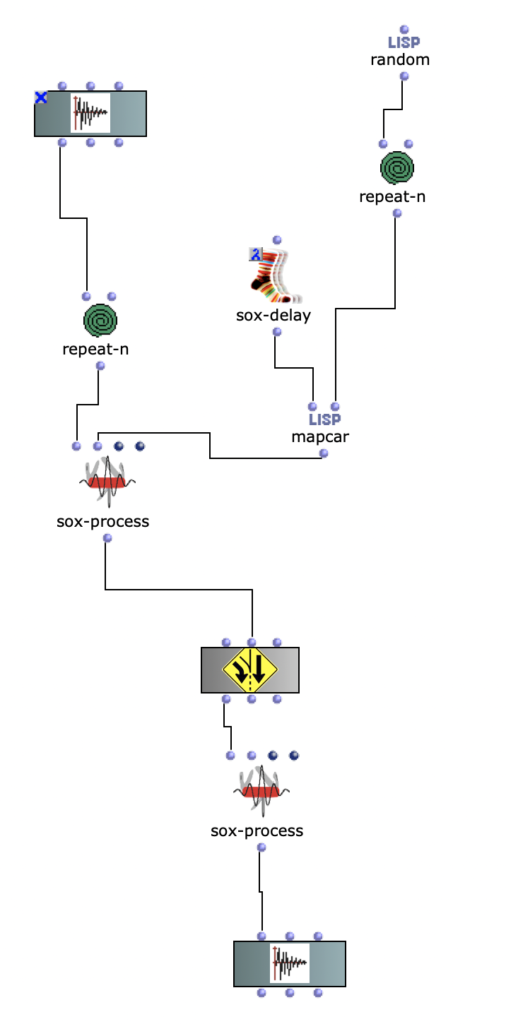
In this iteration, the stereo file was divided into eight speakers.
The different sections of the stereo composition were extracted and different splitting techniques were used.
In one of these, a different fade in and fade out was used for each channel.
In an acousmatic version of a composition, this fade in and fade out can be achieved with the controls of a mixer.
A mapcar and repeat-n were used for this purpose.
Random fades for multichannel
The position of the respective channels was changed in the other processes. A delay was used.
A link to download the applications can be found at the end of this blogpost. This project was also presented as a paper at the 2022 International Conference on Technologies for Music Notation and Representation (TENOR 2022).
Modularity in Sound Synthesis Tools
This blogpost walks through the structure and usage of two applications of machine learning (ML) methods for sound notation and synthesis. The first application is a modular sample replacement engine that uses a supervised classification algorithm to segment and transcribe a drum beat, and then reconstruct that same drum beat with different samples. The second application is a texture synthesis engine that uses an unsupervised clustering algorithm to analyze and sort large numbers of audio files.
The applications were developed in OpenMusic using the OM-SoX modular synthesis/analysis framework. This was so that the applications could be as modular as possible. Modular, meaning that they could be customized, extended, and integrated into a user’s own OpenMusic workflow. We believe this modularity offers something new to the community of ML and sound synthesis/analysis tools currently available. The approach to sound synthesis and analysis used here involves reading and querying many separate audio files. Such an approach can be encompassed by the larger term of “corpus-based concatenative synthesis/analysis,” for which there are already several effective tools: the Caterpillar System, Audioguide, and OM-Pursuit. Additionally, OM-AI, ml.*, and zsa.descriptors are existing toolkits that integrate ML methods into Computer-Aided Composition (CAC) environments. While these tools are very precise, the internal workings of them are not immediately clear. By seeking for our applications to be modular, we mean that they can be edited, extended and integrated into existing CAC programs. It also means that they can be opened and up, examined, and reverse-engineered for a user’s own education.
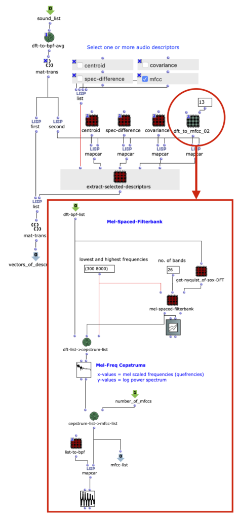
One example of this is in figure 1, our audio analysis engine. Audio descriptors are implemented as subpatches in lambda mode, and can be selected as needed for the input audio.
Figure 1: Interchangeable audio descriptors are set as patches in lambda mode. Here, a patch extracting 13 MFCCs is being used.
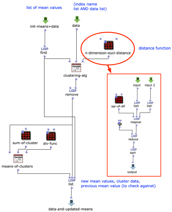
Another example is in figure 2, a customizable distance function in our texture synthesis application. This is the ML clustering algorithm that drives the application. Being a patch built from smaller OpenMusic objects, it is not only a tool for visualizing the algorithm at work, it also allows a user to edit it. For example, the n-dimension euclidean distance function could be substituted with another distance function, if needed.
Figure 2: A simple k-means clustering algorithm, built within an OpenMusic abstraction. The distance function takes the form of a subpatcher in lambda mode.
With the modularity of the project introduced, we will on the next page move on to the two specific applications.
Up until this past August, my impressions of what machine learning could be used for was mostly functional, detached from any aesthetic reference point within my artistic practice. Cars recognizing stop signs, radiologists detecting malignant legions in tissue; these are the first things to come to my mind. There is definitely an art behind programming these tasks. However, it wasn’t clear to me yet how machine learning could relate to my world of contemporary concert music. Therefore, when I participated in Artemi-Maria Gioti’s machine learning workshop at impuls Academy 2021, my primary interest was to make personal artistic connections to this body of research, and to see what ways I could interrogate my underlying aesthetic assumptions in artistic applications of machine learning. The purpose of this text is to share with you the connections I made. I will walk through the composition process of my piece Shepherd for voice and live electronics, using it as a frame to touch upon basic machine learning theories and methods, as well as outline how I aesthetically reacted to them. I will not go deep into the technicalities of machine learning – there are far more qualified people than I for that specific task. However, I will say that the technical content of this blogpost is inspired heavily from Artemi-Maria Gioti, who led this workshop and whose research covers the creative applications of machine learning in a much deeper way. A further dive into the already rich world of machine learning and music can be begun at her website.
A fundamental definition of machine learning can be framed around the idea of improvement through experience. As computer scientist Tom M. Mitchell describes it, “The field of machine learning is concerned with the question of how to construct computer programs that automatically improve with experience.” (Mitchell, T. (1998). Machine Learning. McGraw-Hill.). This premise of ‘improvement’ already confronted me with non-trivial questions. For example, if machine learning is utilized to create an improvising duo partner, what exactly does the computer understand as ‘good’ or ‘bad’ improvisation, as it gains experience? Before even beginning to build a robust machine learning algorithm, answering this preliminary question is an entire undertaking in and of itself. In my piece Shepherd, the electronics were trained to recognize the sound of my voice, specifically whether I was whispering, talking, yelling, or being silent. However, my goal was not to create a perfectly accurate recognition algorithm. Rather, I wanted the effectiveness and the ineffectiveness of the algorithm to both play equal roles in achieving the piece’s concept. Shepherd is a performance piece takes after a metaphor from Jesus in the christian bible – sheep recognize a shepherd by the sound of their voice (John 10). The electronics reacts to my voice in a way that is simultaneously certain and uncertain. It is a reflection, through performance, on the nuances of spiritual faith, the way uncertainty necessarily partakes in the formation of conviction and belief. Here the electronics were not functional instrument (something designed to be controlled by my voice), but rather were functioning more as a second player (a duo partner, reacting to my voice with a level of unpredictability).
Concretely in the program, the electronics returned two separate answers for every input it is given (see figure 1). It gives a decisive, classification answer (“this is ‘silence’, this is ‘whispering’, this is ‘talking’, etc.), and it gives an indecisive, erratic answer via regression (‘silence: 0.833; whispering: 0.126; talking: 0.201; yelling: 0.044’). And important for this concept of conceiving belief through doubt, the classification answer is derived from the regression answer. The decisive answer (classification) was generally stable in its changes over time, while the indecisive answer (regression) moved more quickly and erratically. Overall, this provided a useful material for creating dynamic control of the actual digital sounds that the electronics produced. But before touching on the DSP, I want to outline how exactly these machine learning algorithms operate, how the electronics learn and evaluate the sound of my voice.
Figure 1: Max MSP and Wekinator (off-screen) analyze an audio’s MFCCs to give two outputs on the nature of the input audio. The first output is from a regression algorithm, the second is from a classification algorithm.
In order for the electronics to evaluate my input voice, it first needs a training set, a collection of data extracted from audio of my voice, with which it could use to ‘learn’ my voice. An important technical point is that the machine learning algorithm never observes actual audio data. With training and testing data, the algorithm is always looking at numerical data (here called ‘descriptors’) extracted from the audio. This is one reason machine learning algorithms can work in realtime, even with audio. As I alluded to, my voice recognition program is underpinned by two machine learning concepts: classification and regression. A classification algorithm will return a discrete value from its input data. In my case, those values are ‘silence’, ‘whispering’, ’talking’, and ‘yelling’. To make a training set then, I recorded audio of each of these classes (4 audio files in total), and extracted MFCCs (Mel-Frequency Cepstrum Coefficients) from it. MFCC’s are a representation a sound’s spectral energy calibrated to the range of typical human auditory perception, and are already commonly used in speech recognition programs, music-information retrieval applications, and other applications based around timbre-recognition.
I used the Max MSP library Zsa.descriptors to calculate my MFCCs. I also experimented with other audio descriptors such as spectral centroid, spectral flatness, amplitude peaks, as well as varying numbers of MFCC’s. Eventually I discovered that my algorithm was most accurate when 13 MFCCs were the only descriptor, and that description data was taken only about fivetimes a second. I realized that, on a micro-level timescale, my four classes had a lot similarity. For example, the word ‘synthesizer,’ carried lots of ’s’ noise, which is virtually the same when whispered as when talked. Because of this, extracting data at an intentionally slower rate gave the algorithm a more general picture of each of my voice-classes, allowing these micro-moments of similarity to be smoothed out.
The standard algorithm used for my voice recognition concept was classification. However, my classification algorithm was actually built using a second common machine learning algorithm: regression. As I mentioned before, I wanted to build into my electronics a level of ‘indecision’, something erratic that would contrast the stable nature of a standard classification algorithm. Rather than returning discrete values, a regression algorithm gives a new ‘predictive’ value, based on a function derived from the training set data. In the context of my piece, the regression algorithm does not return a specific voice-class. Rather, it gives four percentage values, each corresponding to how close or far my input is to each of the four voice-classes. Therefore, though I may be whispering, the algorithm does not say whether I am whispering or not. It merely tells me how close or far away I am from the ‘whispering’ data that it has been trained on.
I used a regression algorithm in Wekinator, a simple and powerful machine learning tool, to build my model (see figure 2). Input audio was analyzed in Max MSP, and the descriptor data was sent via OSC to Wekinator. Wekinator built the predictive regression model from this data and then sent output back to Max MSP to be used for DSP control. In Max, I made my own version of a classification algorithm based on this regression data.
Figure 2: Wekinator is evaluating MFCC data from Max MSP and returning 4 values from 0.0-1.0, indicating the input’s similarity to the four voice classes (silence, whispering, talking, yelling). The evaluation is a regression model trained on 752 data samples.
All this algorithm-building once again returns me to my original concern. How can I make an aesthetic connection with these concepts? As I mentioned, this piece, Shepherd is for my solo voice and live electronics. In the piece I stand alone on a stage, switching through different fictional personas (a speaker at a farming convention, a disgruntled restaurant chef, a compilation video of Danny Wolfers saying the word ‘synthesizer,’ and a preacher), and the electronics reacts to these different characters by switching through its own set of personas (sheep; a whispering, whimpering sous chef; a literal synthesizer; and a compilation of christian music). Both the electronics and I change our personas in reaction to each other. I exercise some level control over the electronics, but not total. As I said earlier, the performance of the piece is a reflection on the intertwinement of conviction and doubt, decision and indecision, within spiritual faith. Within this concept, the idea of a machine ‘improving’ towards ‘perfection’ is no longer an effective framework. In the concept, and consequently in the music I attempted to make, stable belief (classification) and unstable indecision (regression) were equal contributors towards the musical relationship between myself and the electronics.
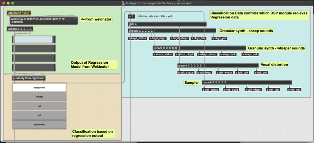
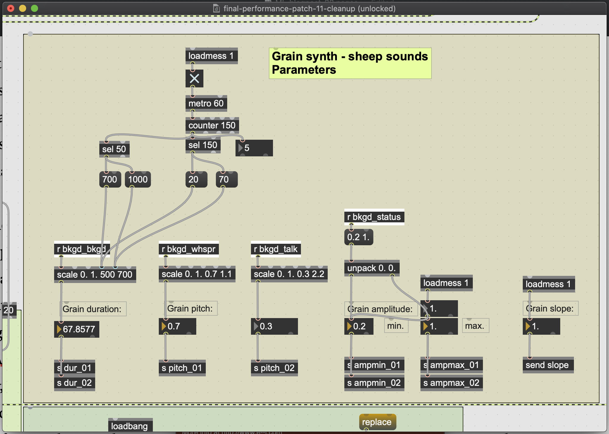
Based on how my voice was classified, the electronics operated one of four DSP modules. The individual parameters of a given module were controlled by the erratic output data of the regression algorithm (see figure 3). For example, when my voice was classified as silent, a granular synthesizer would create textures of sheep-like noises. Within that synthesizer, the percentage levels of whispering and talking ‘detected’ within the silence would manipulate the pitch shifting in the synthesizer (see figure 4). In this way, the music was not just four distinct sound modules. The regression algorithm allowed for each module to bend and flex in certain directions, as my voice subtly suggested hints of one voice class from within another. For example, in one section I alternate rapidly between the persona of a farmer talking at a farming convention, and a chef frustratingly whispering at his sous chef. The electronics moved consequently between my whispering and talking DSP modules. But also, as my whispering became more frustrated and exasperated, the electronics would output higher levels of talking in its regression algorithm. Thus, the internal drama of my theatricalperformances is reacted to by the electronics.
Figure 3: The classification data would trigger one of four DSP modules. A given DSP module would receive the regression values for all four vocal classes. These four values would control the parameters of the DSP module.
Figure 4: Parameter window for granular synth triggered when the electronics classifies my voice as ‘silent’. The amount of whispering and talking detected in the silence would control the pitch of the grain. The amount of silence detected in the silence controlled the grain’s duration. Because this value is relatively static during actual silence from my voice, a level of artificial duration manipulation (seen a the top of the window) was programmed.
I want to return to Tom Mitchell’s thesis that machine learning involves computer improvingautomatically through experience. If Shepherd is a voice recognition tool, then it is inefficient at improvement. However, Shepherd was not conceived as a tool. Rather, creating Shepherd was more so a cultivation of a relationship between my voice and the electronics. The electronics were more of a duo partner, and less of an instrument. To put this more concretely, I was never looking for ‘accurate’ results from the machine. As I programmed, I was searching for results that illustrated Shepherd’s artistic concept of belief intertwined with doubt. In this way, ‘improving’ the piece did not mean improving the algorithm’s accuracy. It meant ‘improving’ the relationship between myself and the electronics. One positive from this approach is that the compositional process was never separated from the programming of the electronics. Both developed in tandem. The composing this piece brought me to the realization that creative applications of machine learning can be applied at every level of its discourse. If you ware interested in hearing a recording of this performance, a bootleg recording of the premiere can be found here.
https://youtu.be/LFQnpp5Uzbg
References:
Artemi-Maria Gioti – composer and artistic researcher working in the field of artificial intelligence.
Wekinator – free, open-source software created by Rebecca Fiebrink that uses machine learning to create musical instruments, game interfaces, computervision, and other tools in sound and animation.
Zsa.descriptors – library for real-time sound descriptors analysis for Max MSP developed by Mikhail Malt and Emmanuel Jourdan.