Yearly Archive July 14, 2024

Byadmin

Music and Installation Chair @IEEE IoS 2024

Marlon Schumacher will serve as music and installation co-chair together with Esther Fee Feichtner for the IEEE

5th International Symposium on the Internet of Sounds

held at the International Audio Laboratories Erlangen, from 30 September – 2 October 2024. Follow this link to the official IEEE Website:

“The Internet of Sounds is an emerging research field at the intersection of the Sound and Music Computing and the Internet of Things domains.  […] The aim is to bring together academics and industry to investigate and advance the development of Internet of Sounds technologies by using novel tools and processes. The event will consist of presentations, keynotes, panels, poster presentations, demonstrations, tutorials, music performances, and installations.”


The Internet of Sounds Research Network is supported by an impressive number (> 120) of institutions from over 20 countries, with a dedicated IEEE committee for emerging technology initiatives. Partners from Germany include:

Byadmin

Trajectory Descriptors: Music Genre Classification through the Tonnetz

Abstract

We present an approach to geometrically represent and analyze the harmonic content of musical compositions based on a formalization of chord sequences as spatial trajectories. This allows us in particular to introduce a toolbox of novel descriptors for automatic music genre classification. Our analysis method first of all implies the definition of harmonic trajectories as curves in a type of geometric pitch class spaces called Tonnetz. We define such curves by representing successive chords appearing in chord progressions as points in the Tonnetz and by connecting consecutive points by geodesic segments. Following a recently established hypothesis that assumes the existence of a narrow link between the musical genre of a work and specific geometric properties of its spatial representation, we introduce a toolbox of descriptors relating to various geometric aspects of the harmonic trajectories. We then assess the appropriateness of these descriptors as a classification tool that we test on compositions belonging to different musical genres. In a further step, we define a representation of transitions between two consecutive chords appearing in a harmonic progression by vectors in the Tonnetz. This allows us to introduce an additional classification method based on this vectorial representation of chord transitions.


Video Presentation:


Conference Article:

SMC2024_paper_id178


This work has been developed as part of the doctoral studies of Christophe Weis and is published in the Proceedings of the Sound and Music Computing Conference 2024 in Porto, Portugal.

ByLukas Körfer

Wave field synthesis with OM-SoX

Abstract: This final project was created at the end of the winter semester 2023/24 as part of the course “Symbolische Klangverarbeitung und Analyse/Synthese” (eng. Symbolic Sound Processing and Analysis/Synthesis) of the MA Music Informatics. An application for sound spatialization was developed in the program OpenMusic using the library OM-SoX implementing Steinberg and Snow’s “acoustic curtain”, a technique for wave field synthesis.

Responsible: Lukas Körfer

Wave field synthesis

Wave field synthesis (WFS for short) is the spatialization of virtual sound sources using a high-density loudspeaker array. This spatialization technique attempts to reproduce a physical soundfield over an extended area in a way to provide for multiple non-conicident listening positions a congruent impression of the localization of sound sources. This is achieved by generating a wave field consisting of a large number of individual sound sources that are synchronized in such a way that a coherent sound wave is created, for which given certain constraints it should be possible to localize a virtual sound source in the room.


For a better understanding of how WFS works, the subject can be approached via the physical phenomenon of interference pattern formation behind an obstacle with openings. When a wave encounters one or more slits, it is diffracted through the openings and propagates behind the obstacle. This leads to the formation of a pattern of wave interference on the other side of the obstacle. Similarly, wave field synthesis uses an array of loudspeakers to generate a coherent sound wave. This requires precise calculation and control of the phase and amplitude relationships of the sound waves emanating from each speaker. These calculations are dependent on the distances of each individual loudspeaker in the array relative to the position in space of the respective virtual sound source.

Project description

For this project, a program was to be created with the general goal of ultimately obtaining a multi-channel audio file that can be used for wave field synthesis with a loudspeaker array through certain influence and adjustments by a user. To achieve this, it was first necessary to design which parameters should be set and influenced by the user of the program.

User input


In addition to the audio file, which is to be used for spatialization, the user must specify certain information about the loudspeaker array on the one hand and the position or positions of one or more virtual sound sources relative to the loudspeaker array on the other. In order to make the configuration of the program as simple and intuitive as possible, I have decided to mainly use a picture object in which the structure can be recorded. The positions of the loudspeakers can be specified by drawing a rectangle and those of the virtual sound sources with circles. One or more circles can be drawn, with each circle representing a sound source. The loudspeakers can be specified in two different ways. If only a single rectangle is drawn in the picture object, this represents the area of a loudspeaker array. In order to be able to determine the specific positions of the individual loudspeakers in the next step of the program, two additional pieces of information are required. Firstly, the length of the loudspeaker array in meters; this also influences the scale for the complete drawn setup. Secondly, the number of loudspeakers in the drawn area must be specified. As soon as more than one rectangle is specified by the user, each individual rectangle represents an individual loudspeaker. In order to be able to specify a scale for the drawn structure in this variant – which was previously possible by specifying the length of the loudspeaker array – the width/height of the area of the complete picture object can now be specified. The first variant, where the loudspeaker array can only be drawn with a rectangle, makes the application much less complicated, but also requires the loudspeakers to be linear and evenly spaced.

Calculating distances


Once all the graphics of the picture object have been read out, they must be divided into rectangles and circles for further processing. If only one rectangle is found, the position and dimension of the rectangle and the two specifications for the length and number of loudspeaker arrays can first be used to determine the position of each individual loudspeaker within the array in meters. If there are several rectangles, this step is not necessary and the center points of all specified rectangles are simply determined. It is then possible to calculate the Euclidean distance from all sources to each individual loudspeaker on the same scale using another Lisp function. It should be noted that all graphics drawn by the user in the Picture object that do not correspond to a rectangle or a circle are ignored and not taken into account for the further calculations. As any number of virtual sound sources can be specified for the application, all circles that exist in the picture object are also captured in this step, whereby the order is irrelevant.

Sound processing


Sound processing is implemented in the next section of the program. Basically, a multi-channel file is created with the sound file specified by the user together with the previously calculated distances, which can be used for the intended loudspeaker array. This process takes place in a nested OM loop with two levels.


In the first level, it is first iterated over each element within the distance list. Each of these elements corresponds to a list that belongs to a virtual sound source, which contains the distances to each loudspeaker. Before the process enters the second level of the loop, further calculations are performed in a Lisp function using the current distance list.

This function iterates over each distance and determines the time delay, volume reduction and a cutoff frequency for a lowpass filter to calculate the air absorption of high frequencies and collects them in a list. In the next step, the result of this Lisp function is used to enter the second level of the loop.


Here, the respective SoX effect is applied to the calculated value; SoX level for volume reduction, SoX lowpass for air absorption and SoX pad for the time delay. The resulting audio file is saved for each iteration. Each of the three lists has as many values as the previously calculated distances from the current sound source to the speakers. This means that each audio file saved in this loop represents one channel of the subsequent multi-channel file for the current sound source.

The multi-channel file can now be created in the next step in the first layer with SoX-Merge and stored temporarily at the end of the loop. This process is repeated for all remaining virtual sound sources (if existing) and are collected as the output of this upper loop. All multi-channel files of the respective sound sources are then merged with a SoX-Mix.

If only one virtual sound source is specified by the user, the output of the outermost loop will only consist of a single multi-channel file for this one source. In this case, the SoX-Mix is not required and it would even lead to an error during the evaluation of the program if the input of the SoX-Mix consisted of only one audio file. The OM-If therefore avoids the use of the SoX-Mix as soon as the output of the patcher, in which the distances are determined, only consists of one list, which means that only one circle for a virtual sound source has been drawn in the picture object.

Finally, silence can be added to the multi-channel file using the SoX pad, depending on preference, if the selected audio file is particularly short, for example. At the same time, the final multi-channel file is saved in Outfile as “wfsOutFile.wav”.

ByFlorian Simon

Interspaces – Acousmatic study with OM-SoX

Interspaces juxtaposes sounds from human civilization with sounds from nature. Four pairs of field recordings are presented, which are filtered according to the principle of a vocoder according to the spectrum of a section of the counterpart.

Responsible: Florian Simon

Interspaces shows the following four pairs (format: total recording – source of the spectrum):

  1. Chirping Arctic terns – Vowel “E” called by humans
    Lively market, people talking and calling – Arctic tern call

  2. Rippling of a river – Accelerating car
    Main road – rushing of a river

  3. Forest scenery, rustling leaves and birds – Train horn
    Station concourse – chirping of a songbird

  4. Thunderstorm – clinking of cutlery
    Business in a restaurant kitchen – thunder

The field recordings come from the FreeToUseSounds library.

Interspaces uses an equilateral octagonal loudspeaker arrangement, whereby the two channels of the source material are each placed at opposite points in the array. The two recordings of a pair are also offset by 90 degrees from each other by default, so that four sound sources can be perceived.

Each recording is divided into several sections of random size within a certain frame and concatenated again in randomized order with short crossfades. The number of sections increases with each pair of recordings: 4, 9, 16 and finally 23. With each new section, the two sound sources also “move” in the array by 0.25 channels in a certain direction. Since the number of sections is the same for both recordings of a pair, but not the position of the cuts, deviations from the base of a 90-degree spacing and a greater variety of sounds are created. Interspaces is designed as an installation to allow free exploration of the stereo fields.

Interspaces was created in OpenMusic using functions from the OM-SoX library. The underlying program consists of two parts. The first is used to create the manipulated recordings by spectral analysis (sox-dft), splitting the source material into up to 4096 frequency bands (sox-sinc), adjusting their volume levels according to the generated spectrum (sox-level) and reassembling them (sox-mix).

The second part of the program uses the synthesis patch of a maquette to control the division into sections (sox-trim) and their spatialization (sox-remix) and final alignment (sox-splice) for each of the eight generated audio files, and finally to organize the finished blocks in terms of time (sox-pad and sox-mix). In the last step, the time saved by the crossfades must be taken into account and subtracted from the onset value/x position in the maquette.

Audio (binaural mixed to stereo):


Unfortunately, this vocoder method has the disadvantage that the individual frequency bands are initially very quiet and therefore artefacts in the form of noise occur when applying the gain and the final normalization. Conversely, clipping occurs when certain frequencies are strongly represented in both source recordings. If you lower the gain values accordingly to avoid this, quieter sections in the result may be barely audible, depending on the size of the dynamic difference. The noise can be easily eliminated by selecting higher gain values, but this increases the clipping problem. In the above version of Interspaces, the best compromise between the two effects was sought for all eight audio clips.


ByAlexander Vozian

Co-Creative Melody Generator: Visual Live-Coding with OM and Supercollider

Abstract: The Co-Creative Melody Generator is a system for simultaneous live coding with SuperCollider and OpenMusic. While in OpenMusic the music is created at note level, SuperCollider is responsible for sound generation. Communication takes place through the exchange of messages in the Open Sound Control protocol via user queries or automatically.

Responsible persons: Alexander Vozian

Overview:

The goal of the project was to integrate OpenMusic (OM) into a live coding workflow. My first idea was to use SuperCollider (SC) for sound generation and to outsource the setting of notes to OM. This means that you can code live in SC and use OM as an auxiliary tool. However, it became clear during the development that the OM patch can be changed in parallel during the sound output. As long as the sound-generating element is not interrupted, live coding can also take place in OM. For example, it is possible to prepare the selection of “instruments”, in this case SC synths, and control them completely in OM. Another more collaborative approach would be to split the two programs, SC and OM, between two live coders. For example, one person in SC could do the sound design, while another in OM sets these sounds in time.

OM takes care of generating the notes and SC takes care of the sound synthesis. These communicate via the Open Sound Control (OSC) protocol. In SC, the user (live coder) sends a request to the OM patch via an OSC message. The message contains parameters for the generation of a melody, in this case for a Markov analysis and synthesis. The message consists of:

  • the maximum number of notes,
  • the maximum length of a loop in ms,
  • the lower and upper limit of the source material to be analyzed in ms
  • Selection of the source material.

The source material is a midi file, about 1 min long.

Sources of the midi files: bitmidi.com

After synthesis, OM automatically sends a message with the number of notes generated, the length of the melody in ms, a list of frequencies and a list of onsets. These are used to control the synths in SC.

With each evaluation, note material is analyzed and a list of frequencies and onsets is synthesized and then output.

Midi files about 1 min long are used to generate the notes. The pitches and durations of the notes are analyzed independently of each other using first-order Markov functions from the OM-Alea library, synthesized and sent via osc-send. This results in tone sequences that do not occur in the original files. (The patch ensures that the list of pitches and durations is the same length) The input arguments are already described above.

An OSC message from OM to SC consists of the following data:

  • OSC Key as identifier,
  • Total number of notes,
  • Length of the melody in milliseconds,
  • List of frequencies,
  • List of onsets.

In this case, the total number of notes is only used to navigate through the unformatted OSC message. The length of the melody is required to determine the time at which the next melody is requested. The list of frequencies and onsets is only compiled in SC.

The osc-send function is in the patch markov_firstorder_osc_send. To execute the patch automatically when an OSC message arrives, all parts of the higher-level patch are set to reactive mode. The list function can only be evaluated when all forms deliver a result, i.e. when the Markov synthesis has been completed and osc-send has been executed.

The result is a kind of server that automatically sends back a melody when a request is received from SC.

A new instance of OSCdef is created in SC, which saves the parameters received in global variables. A synth(t1) is defined that can be played by patterns. The Pfuncn function interprets the global variables ~freq and ~dur as functions and thus constantly queries them. The Pseq function converts these into a sequence, which is converted into a pattern by Pbind. Thus, the first parameter of ~freq with the first parameter of ~dur forms the first note of the melody. The Pdef function creates an instance that can be changed during runtime. This also ensures that a running loop only plays a new melody after the end of a melody.

To request a new melody, a new loop, it is sufficient to send an OSC message with the corresponding parameters. To automate this process, you need the Tdef.

Just as the execution of a code block in SC can have a direct influence on the sound and must therefore be embedded correctly, the evaluation of a patch must take place at the right time. In the case of the MWE, it is not the sound that would be interrupted, but the meter.

Tdef(om) first calculates the time period with which the sending of the OSC message is delayed. The delay time depends on the total length of the loop and the number of loops that can be set within the Tdef. This ensures that the existing loop is always played to the end before the parameters for a new melody arrive.

The code for OM and SC can be found via this link.

Finally, the following sound example for the project:

Only the maximum length of a loop and the number of notes are changed. The source material is changed at two points. It starts with “Mario”, changes at around 1:39 to “Pokemon” and at 2:24 to “Tetris”. In the example, nothing is deliberately changed in the sound of the instrument (simple saw wave) in order to focus on the changes in the note material.

Mario – Main Theme Overworld:


Pokemon – Battle (vs Wild Pokémon):


Tetris Theme:


Result:

Sources of the midi files: bitmidi.com

ByFlorian Simon

PixelWaltz: Sonification of images in OpenMusic

Abstract: The OpenMusic program PixelWaltz can be used to convert images into symbolic representations of music (pitches and onset times). Options for image manipulation are available with which the result can be additionally influenced.

Responsible persons: Florian Simon

Mapping: Pitch

The pixels of the image are scrolled through line by line and the respective red, green and blue values (between 0 and 1) are mapped to a desired pitch range. This means that three pitch values in midicent are always obtained from one pixel. As two adjacent pixels are similar in many cases, this mapping method often results in repeating patterns every three notes. This is the reason for the title of the project.

It is also possible to limit the number of note values output.

Mapping: Application times

A constant value can be set for the start times and note durations. A humanizer effect can also be switched on, which randomly shifts each note forwards or backwards within a specified range. Starting from the basic tempo, accelerandi and ritardandi can be created by passing lists of three numbers. These represent the start note, end note and speed of the tempo change. (20 50 -1) creates an accelerando from note 20 to note 50, in which the intervals per note become one millisecond shorter. A positive third value corresponds to a ritardando.

Dynamics

Different random ranges for “red”, “green” and “blue” notes can be defined for the volume or velocity. The values generated in this way can also be modulated sinusoidally so that, for example, the volume can rise and fall over longer periods of time. This requires the specification of a wavelength in the number of notes and the maximum deviation factor.

Accompaniment

PixelWaltz offers the option of generating an accompanying voice, which consists of individual additional tones in a desired fixed note number frequency. If this is not divisible by 3, a polymetric is often created. The pitch is determined randomly and can be between 3 and 6 semitones below the respective “accompanied” note.

Image processing

In order to create further variation, the sonification section of PixelWaltz is preceded by tools for manipulating the input image. In addition to adjusting the image size, brightness and contrast, it is also possible to shift the color values and thus recolor the image. The changes in the musical translation are immediately noticeable: More brightness leads to a higher average pitch, more contrast reduces the number of different pitch values. With a blue-dominated image, the last notes of the triplet will usually be the highest.

Sound results

The tonal results naturally differ depending on the input – but photographed material in particular often leads to the same wave-like overall structure, which winds irregularly and at a slow tempo chromatically, sometimes upwards, sometimes downwards. The accompaniment supports this effect and can form a counter-pulse to the main voice.

ByLaura Peter

Whitney Music Box with OMChroma/OMPrisma in OpenMusic

The Whitney Music Box is a sonified and/or visual representation of a series of interrelated sound elements. From a musical point of view, these elements can be related chromatically or harmonically, for example. In the visual representation, each of these elements is represented by a circle or dot (see Figure 1). These dots circle around a common center point depending on their own assigned frequency. The lower the frequency, the smaller the radius of the orbiting circle and the higher the orbital speed. Each sound element represents multiples of a fixed fundamental frequency in a harmonic series. As soon as an element has completed a revolution around the center point, the sound is triggered with the frequency it represents. Due to the mathematical relationship between the individual elements, there are moments during the performance of the Whitney Music Box in which certain elements are triggered simultaneously and phases in which the elements can be perceived consecutively. At the beginning and at the end, all elements are triggered simultaneously.

Figure 1: Whitney Music Box – visual representation

In this project, OMChroma is used to synthesize the individual sound elements (see Figure 2). The synthesis classes of OMChroma inherit from OpenMusic’s class-array object. The columns in the array describe the individual components within the synthesis. The rows represent parameters that can be assigned locally to the individual components or globally to the entire process. For the Whitney Music Box, elements are needed that implement the individual pitch gradations and the temporal offset of the individual pitch gradations. An OMChroma matrix is regarded as an event. Such an event represents a pitch and the sound repetitions within the global duration of the Whitney Music Box. The global duration is defined at the beginning and also describes the round trip time of the lowest frequency or the previously defined start frequency. Each matrix represents a frequency that is a multiple of the start frequency. The round trip time of a sound element is calculated using the formula

duration(global) / n

Where n is the index of the individual sound elements or matrices. The higher the index, the higher the frequency and the shorter the round trip time. The repetitions of the sound elements are defined by the parameter e-dels . Each component of a matrix is given a different entry delay. These entry delays are spaced at regular intervals of duration(global) / n.

Figure 2: Application of OMChroma

Without spatialization, the Whitney Music Box with OMChroma sounds like this:


Figure 3 shows how the collected matrices or sound events are spatialized with the OMPrisma library. This was based on the visual representation of the Whitney Music Box. Sound elements with a low frequency are further away from the center and sound elements with a high frequency circle closer to the center. With OMPrisma, this representation is to be implemented in spatial sound. This means that sounds with a low frequency should sound further away and sounds with a high frequency should sound closer to the listener. In the OpenMusic patch, elements with an even index were also positioned further to the front and further to the right and, similarly, elements with an odd index were positioned further to the left and back in order to distribute the sounds evenly in the room. The OMPrisma classes also offer presets for the attenuation function, air-absorption function and time-of-flight function . These were used to create an even greater sense of spatiality in addition to the positioning in the room.

Figure 3: Application of OMPrisma

In stereo, for example, the Whitney Music Box sounds like this:


Figure 4 shows how the collected OMChroma and OMPrisma matrices are merged using the chroma-prisma function. The list of all collected matrices is returned via an om-loop and rendered as a sound using the synthesize function(see Figure 5).

Figure 4: chroma-prisma

Figure 5: loop and synthesize

The OpenMusic patch and sound samples can be downloaded from the following link: https://github.com/lauraptrcodes/Whitney-music-box

ByMoritz Reiser

Markov processes for controlling harmonics in OpenMusic and Common Lisp

Abstract: A project on the use of random processes in a musical context. Basically, two different models are used. These generate chord sequences, which are then provided with a rhythm and an overlying melody.

Responsible: Moritz Reiser


Overview

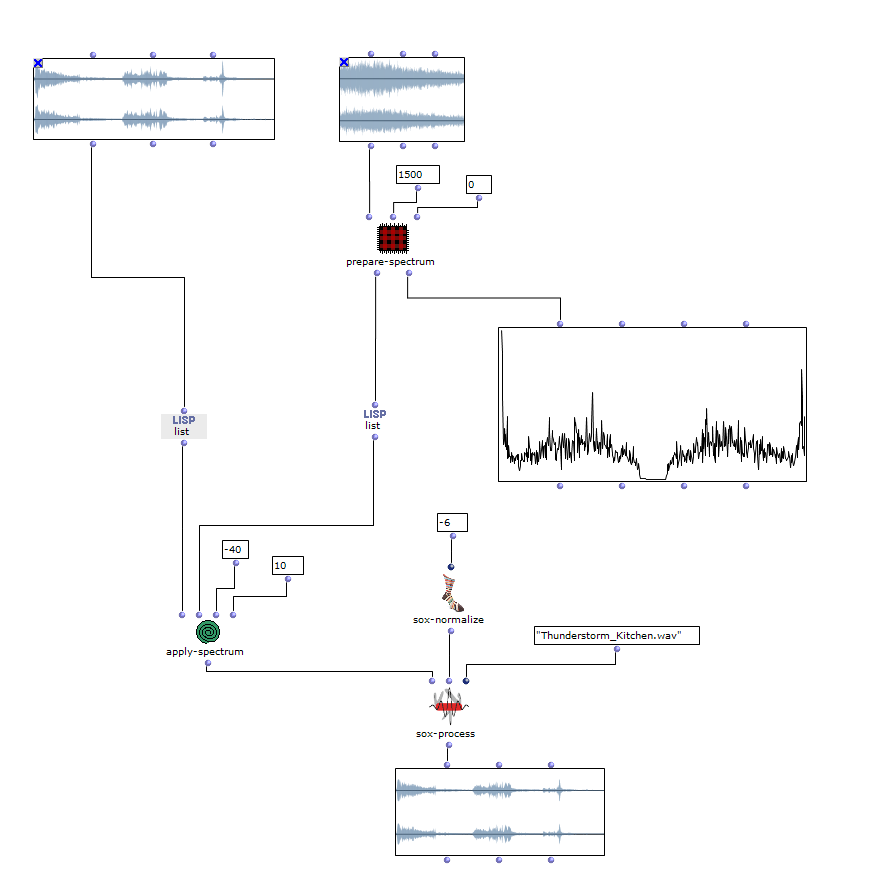
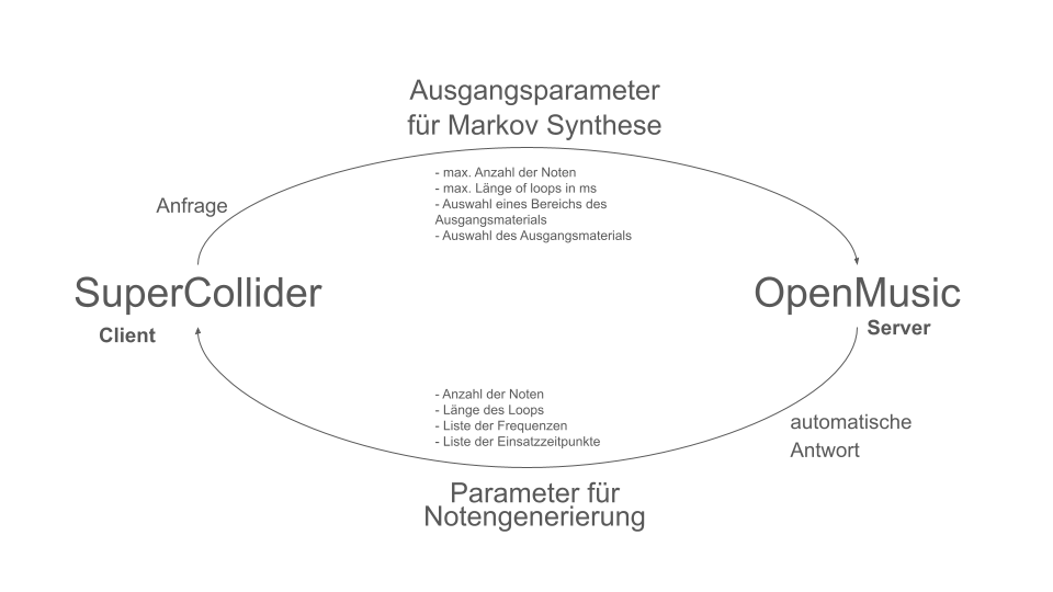
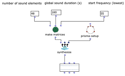
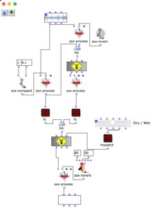
The overall structure of the program, which corresponds to the content of the main patch, can be seen in Figure 1. At the top is the selection of the algorithm to be used for chord progression generation. This can be selected via the selection field at the top left. The two input fields of the subpatches can be used to specify the desired length and the starting chord or the key of the composition.

This is followed by a random determination of the respective tone lengths. Here you can set the tempo in BPM as well as the frequencies of the tone lengths occurring in multiples of quarter notes. The respective start times of the chords are calculated from the calculated durations using a “dx→x” function. When using the program, care must be taken here that Open Music calculates new random numbers in both strings due to the output being used twice, as a result of which the relationship between the start time and the tone duration is lost. This can be remedied by locking the subpatches for chord progression and tone length generation with “Lock Eval” after running the program once and then running it again to adjust the start times to the now saved tone durations (see information panel in the main patch). The third major step in the overall process is the generation of a melody that lies above the chord sequence. Here, a note is selected from the underlying chord and shifted up an octave. You can set whether this should always be a random chord tone or whether the tone closest to or furthest away from the preceding melody tone should be selected.

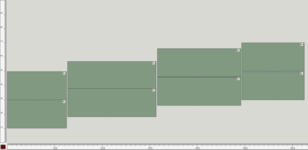
The result is then visualized at the bottom in a multi-seq object.

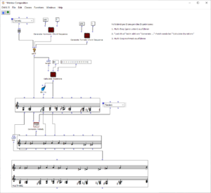
Figure 1: Overall structure of the composition process


Chord progression generation

Two algorithms are available for generating the chord sequence. The desired length of the sequence, which corresponds to the number of chords, and the starting chord or the key are transferred to them.

Harmonic chord sequence using Markov chain

The sequence of the first algorithm can be seen in Figure 2. The subpatch “Create Harmonic Chords” generates the basic set of chords that will be used in the following. This corresponds to the usual levels of counterpoint theory and, in addition to the tonic, subdominant, dominant and their parallels, contains a diminished chord on the seventh degree, a sixth ajoutée of the subdominant and a dominant seventh chord. The “Key” input adds a value corresponding to the desired key to these chords.

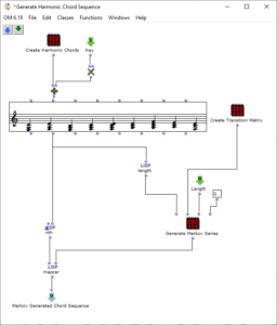
Figure 2: Subpatch for generating a harmonic chord sequence using a Markov chain

The “Create Transition Matrix” subpatch generates a matrix with transition probabilities for the individual chords. For each chord step, the probability with which it transitions to a certain other chord is determined. The probability values were chosen arbitrarily according to the usual processes in counterpoint theory and adjusted experimentally. For each chord it was investigated how likely it is to transition from this chord to another chord, so that the result corresponds to the conventions of counterpoint theory and allows a frequent return to the tonic level in order to focus on it. The exact transition probabilities are listed in the following table, whereby the initial sounds are listed in the left-hand column and the transitions are represented line by line.

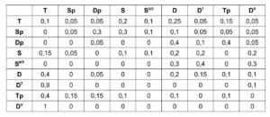
Table 1. Transition probabilities of the harmonies of corresponding chord levels

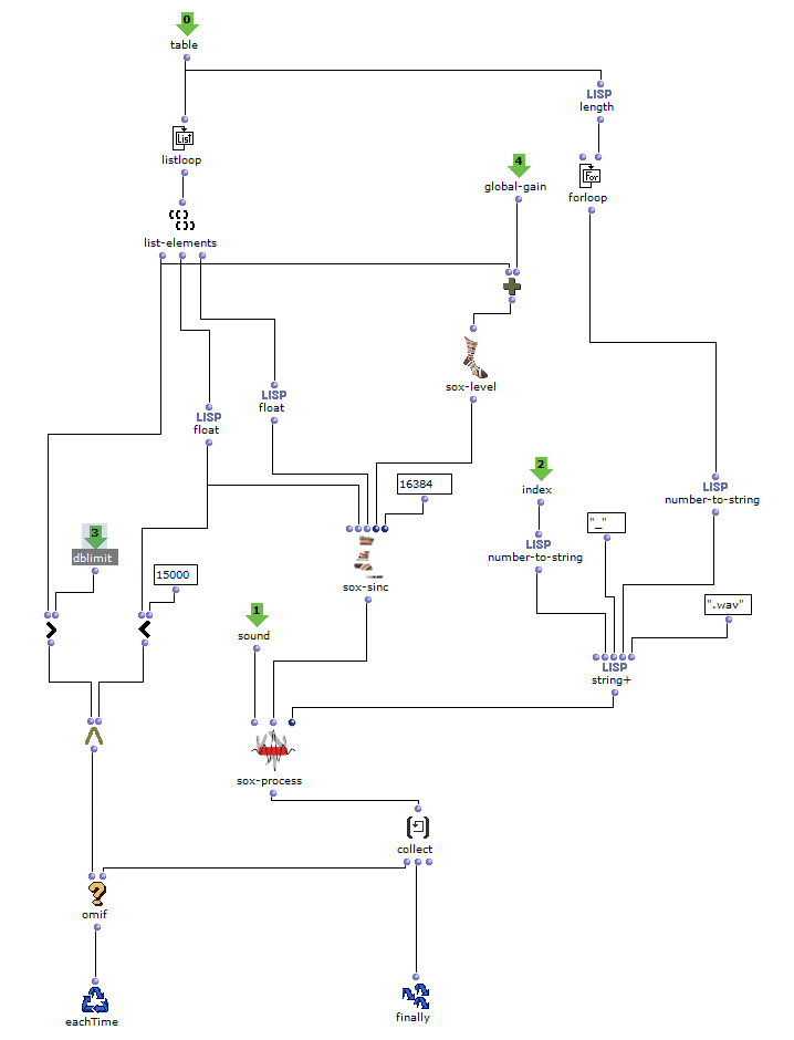
The generation of the chord sequence finally takes place in the patch “Generate Markov Series”, which is shown in Figure 3. This initially only works with the numbering of the chord steps, which is why it is sufficient to pass it the length of the chord list. The Lisp function “Markov Synthesis” now generates a chord sequence of the desired length using the transition matrix. As it is not guaranteed that the last chord in the sequence generated in this way corresponds to the tonic, another Lisp function is used, which generates further chords until the tonic is reached. As the steps have only been numbered so far, the chords valid for the respective steps are finally selected in order to obtain the finished chord sequence.

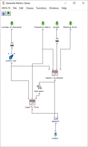
Figure 3: Subpatch for generating a chord sequence using Markov synthesis

 
Chromatic chord progression using a tone net

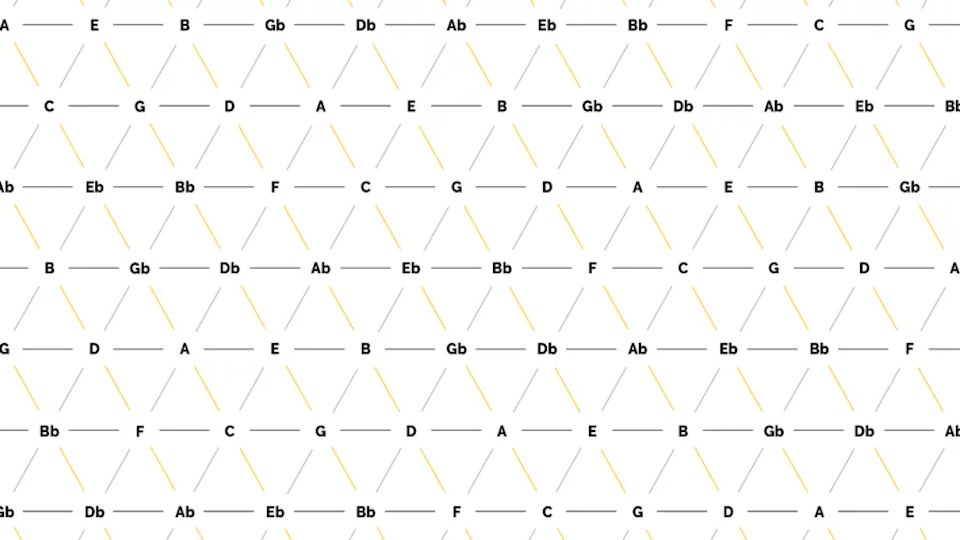
In contrast to the harmonic chord progression, all 24 major and minor chords of the chromatic scale are used here (see Figure 4). The special feature of this algorithm lies in the choice of transition probabilities. These are based on a so-called tone network, which is shown in Figure 5.

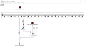
Figure 4: Subpatch for generating a chord sequence based on the tone net representation

Figure 5: Tonnetz (image source:<https://jazz-library.com/articles/tonnetz/>)

Within the tone net, individual tones are applied and connected to each other. On the horizontal lines, the tones are each a fifth apart, while the diagonal lines show minor thirds (from top left to bottom right) and major thirds (from bottom left to top right). The resulting triangles each represent a triad, for example the triangle of the notes C, E and G results in the chord C major. All major and minor chords of the chromatic scale can be found. The Tonnetz representation is mostly used for analysis purposes, as a Tonnetz allows you to see directly how many tones two different triads share. One example is the analysis of classical music of the romantic and modern periods as well as film music, as the harmonic counterpoint rules used above are often neglected here in favor of chromatic and other previously unusual transitions. The distance between two chords in the tonal network can be a measure of whether the transition of one chord into the other is melodious or rather unusual. It is calculated from the number of edges that have to be crossed to get from one chord triangle to another. In other words, it corresponds to the degree of adjacency between two triangles, whereby a direct adjacency results from sharing an edge. Figure 6 shows an example of this: To get from the chord C major to the chord F minor, three edges have to be crossed, resulting in a distance of 3.

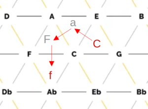
Figure 6: Example of determining the distance in the tone network using the transition from C major to F minor

As part of the project, the transition probabilities are now calculated on the basis of the distances between chords in the tone network. It is only necessary to distinguish whether the active triad is a major or minor chord, as the same distances to other chords result for all keys within these two classes. This means that every transition can be calculated from C major or C minor and then shifted to the desired key by adding a value. Starting from both variants (C major and C minor), the distances to all other triads were first recorded in the tonal network:

Distances from C major:

Intervals from C minor:

In order to obtain probabilities from the intervals, all values were first subtracted from 6 to make larger intervals less probable. The results were then used as the exponent of the number 2 in order to give greater weighting to closer chords. Overall, this results in the formula

P=2^(6-x) ; P=probability, x=distance in the grid

to calculate the transition weights. These result in the following matrix for all possible chord combinations, from which 342 probabilities result when divided by the row sum.

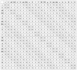
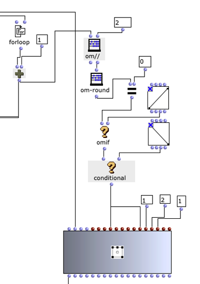
Within the patch, the Lisp function “Generate Tonnetz Series” first determines whether the active chord is a major or minor triad. As with the harmonic procedure, only the numbers 0-23 are used initially, this can be determined using a simple modulo-2 calculation. Depending on the result, the respective probability vector is used, a new chord is determined and finally the previous step is added. If the result is a number greater than 23, 24 is subtracted in order to always remain within the same octave.

After the previously determined length of the sequence, this section is finished. There is no return to the tonic as in the previous section, as the chromaticism means that the tonic is not as pronounced as in the harmonic chord sequence.

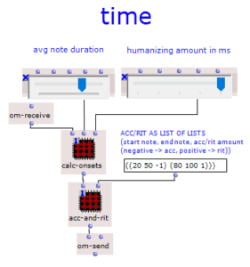
Determining the tone lengths

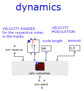
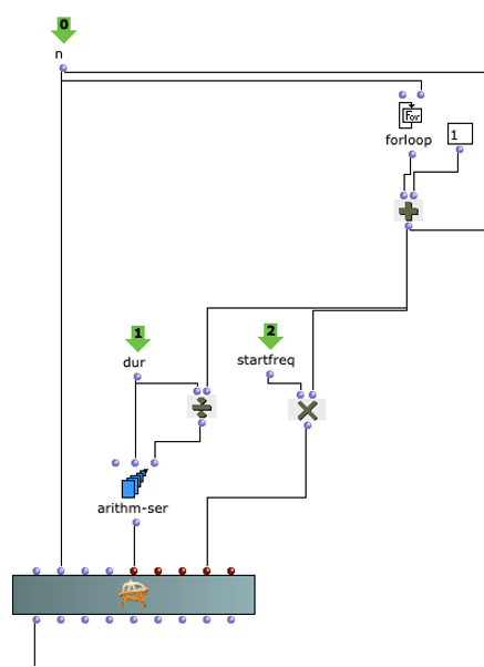
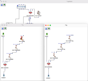
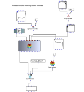
After a chord progression has been generated, random lengths are calculated for the individual triads. This is done in the “Calculate Durations” subpatch, which is shown in Figure 6. In addition to the desired BPM number, a list of note lengths is transferred as multiples of quarter notes. More probable values occur more frequently in this pool, so that a corresponding selection can be made via “nth-random”.

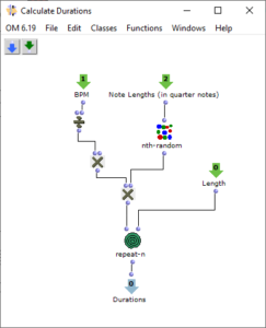
Figure 7: Subpatch for random determination of note durations
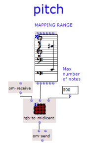
Melody generation

The basic melody generation process has already been described above: A tone is selected from the respective chord and transposed up an octave. This tone can be selected at random or according to the smallest or largest distance to the previous tone.


Sound examples

Example of a harmonic chord sequence:


Example of a tone net chord sequence:


ByAndres Kaufmes

Transient Processor

Transient Processor

SKAS symbolic sound processing and analysis/synthesis

Prof. Dr. Marlon Schumacher

Intermediate project by Andres Kaufmes

HfM Karlsruhe – IMWI (Institute for Music Informatics and Musicology)

Winter semester 2022/23

_____________

For this interim project, I worked on the implementation of a transient processor in OpenMusic with the help of the OM-Sox library.
A transient processor (also known as a transient designer or transient shaper) can be used to influence the attack/release behavior of the transients of an audio signal.

The first hardware device presented was the SPL TD4, introduced by SPL in 1998, which was available as a 19″ rack device and is still available today in an advanced version.

Transient Designer from SPL. (c) SPL

Transient Designers are particularly suitable for processing percussive sounds or speech. First, the transients must be isolated from the desired audio signal; this can be done using a compressor, for example. A short attack time “ducks” the transients and the signal can be subtracted from the original. The audio signal can then be processed with further effects in the course of the signal chain.

Transient processor patch. FX chain of the two signal paths (left “Transient”, right “Residual”).

At the top of the patch you can see the audio file to be processed, from which, as just described, the transients are isolated using a compressor and the resulting signal is subtracted from the original. Now two signal paths are created: The isolated transients are processed in the left-hand “chain”, the residual signal in the right-hand one. After both signal paths have been processed with audio effects, they are mixed together, whereby the mixing ratio (dry/wet) of both signal paths can be adjusted as desired. At the end of the signal processing there is a global reverb effect.

“Scope” view of the two signal paths. Sketches of the possible signal path and processing.

Sound examples:

Isolated signal:

Residual signal:

Byadmin

Spatial transformation of the piece “Ode An Die Reparatur” (“Ode To The Repair”)

Abstract: The entry describes the spatialization of the piece “Ode An Die Reparatur” (“Ode To The Repair”) (2021) and its transformation into a Higher Order Ambisonics version. A binaural mix of the finished piece makes it possible to understand the working process based on the result.

Supervisor: Prof. Dr. Marlon Schumacher

A contribution by: Jakob Schreiber

Piece

The piece “Ode An Die Reparatur” (2021) consists of four movements, each of which refers to a different aspect of a fictional machine. What was interesting about this process was to investigate the transition from machine sounds to musical sounds and to shape it over the course of the piece.

Production

The production resources for the piece were, on the one hand, a UHER tape recorder, which enables simple repitch changes and was predestined for the realization of this piece based on mechanical machines due to its functionality with motors and belts. SuperCollider was also used as a digital sound synthesis and alienation environment.

Structure

The piece consists of four movements.

First movement

The sound material of the beginning is composed of various recordings from a tape recorder, over which clearly audible, synthesized engine sounds are played alongside silence.

Second movement

The sound objects, some of which are reminiscent of birdsong, suddenly emerge from sterile silence into the foreground.

Third movement

The perforative characteristics inside a gearwheel are transformed into tonal resonances in the course of the movement.

Fourth movement

In the last movement, the engines play a monumental final hymn.

Spatialization

Based on the compositional form of the piece, the spatialization drafts adhere to the division into movements.

Working practice

The working process can be divided into different sections, similar to the OM patch. In the laboratory section, I explored different forms of spatialization in terms of their aesthetic effect and examined their conformity with the compositional form of the existing piece.

In order to determine different trajectories, or fixed positions of sound objects, the visual assessment of the respective trajectories played an important role in addition to the auditory effect.

Ultimately, the parameters of the pre-selected trajectories were supplemented with a scattering curve, finely adjusted and finally transformed into a fifth-order Higher Order Ambisonics audio file via a chain of modules.

Iteratively, the synthesized multi-channel files are added to the overall structure in REAPER and their effect is examined before they are run through the synthesis process again with an optimized set of parameters and trajectories.

More details on the individual sentences

First, you can listen to the binaural version of the spatialized piece as a whole. The approaches of the individual parts are described briefly below

 
First sentence

In the first part, the long, drawn-out clouds of sound, lying on top of each other like layers, move according to the basic tempo of the movement. The trajectories lie in a U-shape around the listening area, covering only the sides and front.

Second movement

Individual sound objects should be heard from very different positions. Almost percussive sounds from all directions of the room make the listener’s attention jump.

Third movement

The sonic material of this part is a sound synthesis based on the sound of cogwheels or gears. The focus here was on immersion in the fictitious machine. From this very sound material, resonances and other changes create horizontal tones that are strung together to form short motifs.

The spatialization concept for this part is made up of moving and partly static objects. The moving ones create an impression of spatial immersion at the beginning of the movement. At the end of the movement, two relatively static objects are added to the left and right of the stereo base, which primarily emphasize the melodic aspects of the sound and merely oscillate fleetingly on the vertical axis at their respective positions.

Fourth movement

The instrumentation of this part of the piece consists of three simulations of an electric motor, each of which follows its own voice. In order to separate the individual voices a little better, I decided to treat each of the four motors as an individual sound object. To support the monumental character of the final part, the objects only move very slowly through the fictitious space.