Abstract: This final project was created at the end of the winter semester 2023/24 as part of the course “Symbolische Klangverarbeitung und Analyse/Synthese” (eng. Symbolic Sound Processing and Analysis/Synthesis) of the MA Music Informatics. An application for sound spatialization was developed in the program OpenMusic using the library OM-SoX implementing Steinberg and Snow’s “acoustic curtain”, a technique for wave field synthesis.
Responsible: Lukas Körfer
Wave field synthesis
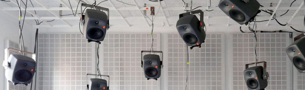
Wave field synthesis (WFS for short) is the spatialization of virtual sound sources using a high-density loudspeaker array. This spatialization technique attempts to reproduce a physical soundfield over an extended area in a way to provide for multiple non-conicident listening positions a congruent impression of the localization of sound sources. This is achieved by generating a wave field consisting of a large number of individual sound sources that are synchronized in such a way that a coherent sound wave is created, for which given certain constraints it should be possible to localize a virtual sound source in the room.
For a better understanding of how WFS works, the subject can be approached via the physical phenomenon of interference pattern formation behind an obstacle with openings. When a wave encounters one or more slits, it is diffracted through the openings and propagates behind the obstacle. This leads to the formation of a pattern of wave interference on the other side of the obstacle. Similarly, wave field synthesis uses an array of loudspeakers to generate a coherent sound wave. This requires precise calculation and control of the phase and amplitude relationships of the sound waves emanating from each speaker. These calculations are dependent on the distances of each individual loudspeaker in the array relative to the position in space of the respective virtual sound source.
Project description
For this project, a program was to be created with the general goal of ultimately obtaining a multi-channel audio file that can be used for wave field synthesis with a loudspeaker array through certain influence and adjustments by a user. To achieve this, it was first necessary to design which parameters should be set and influenced by the user of the program.
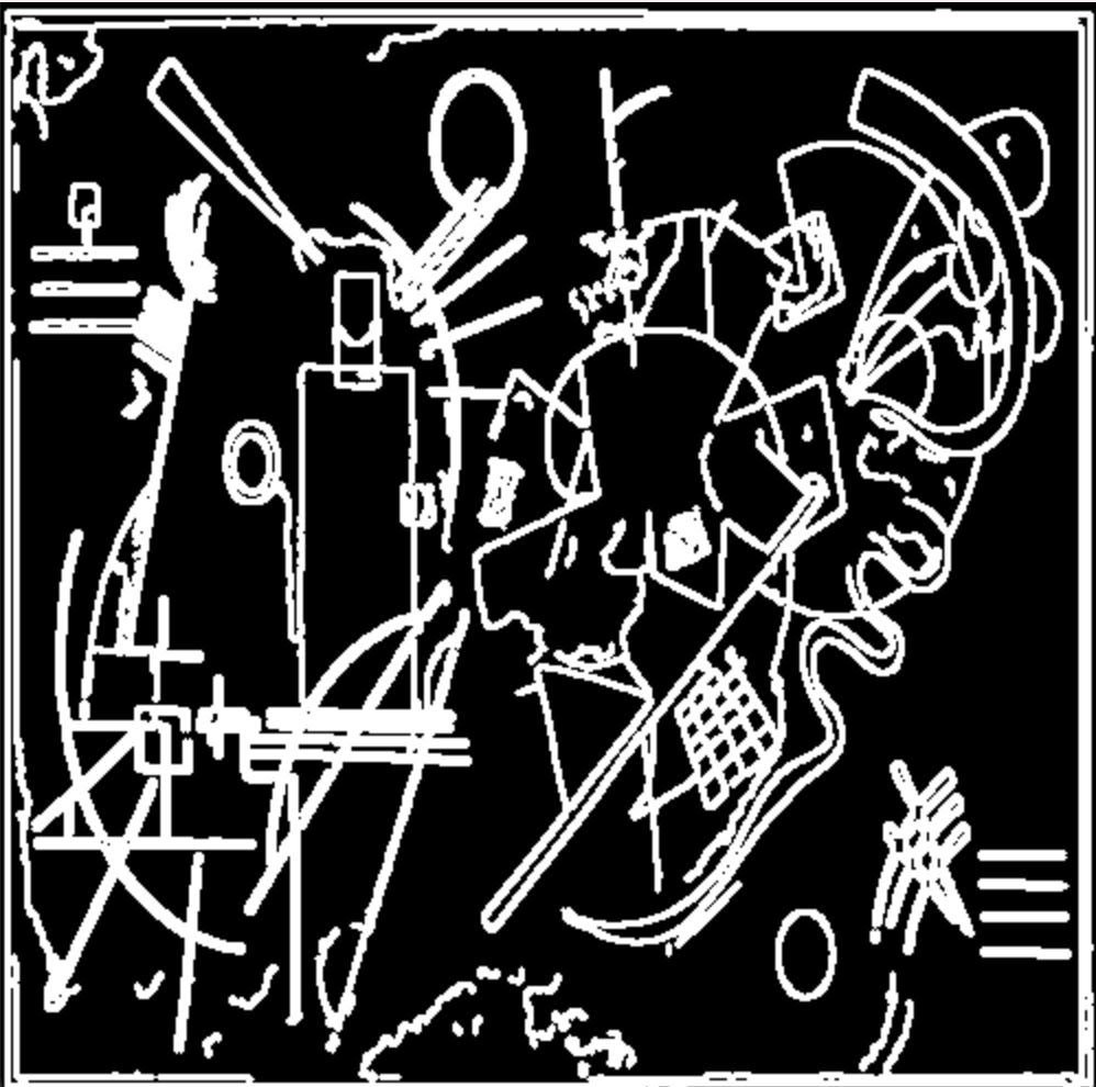
User input
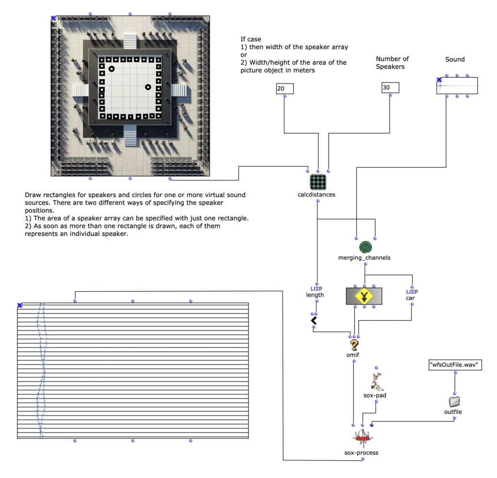
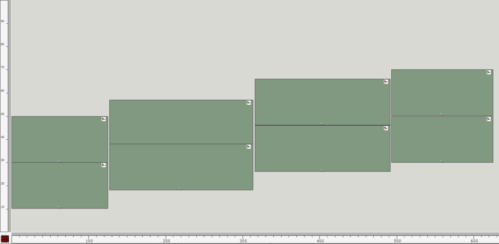
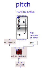
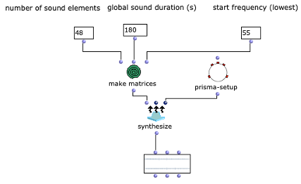
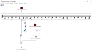
In addition to the audio file, which is to be used for spatialization, the user must specify certain information about the loudspeaker array on the one hand and the position or positions of one or more virtual sound sources relative to the loudspeaker array on the other. In order to make the configuration of the program as simple and intuitive as possible, I have decided to mainly use a picture object in which the structure can be recorded. The positions of the loudspeakers can be specified by drawing a rectangle and those of the virtual sound sources with circles. One or more circles can be drawn, with each circle representing a sound source. The loudspeakers can be specified in two different ways. If only a single rectangle is drawn in the picture object, this represents the area of a loudspeaker array. In order to be able to determine the specific positions of the individual loudspeakers in the next step of the program, two additional pieces of information are required. Firstly, the length of the loudspeaker array in meters; this also influences the scale for the complete drawn setup. Secondly, the number of loudspeakers in the drawn area must be specified. As soon as more than one rectangle is specified by the user, each individual rectangle represents an individual loudspeaker. In order to be able to specify a scale for the drawn structure in this variant – which was previously possible by specifying the length of the loudspeaker array – the width/height of the area of the complete picture object can now be specified. The first variant, where the loudspeaker array can only be drawn with a rectangle, makes the application much less complicated, but also requires the loudspeakers to be linear and evenly spaced.
Calculating distances
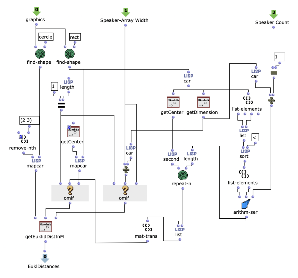
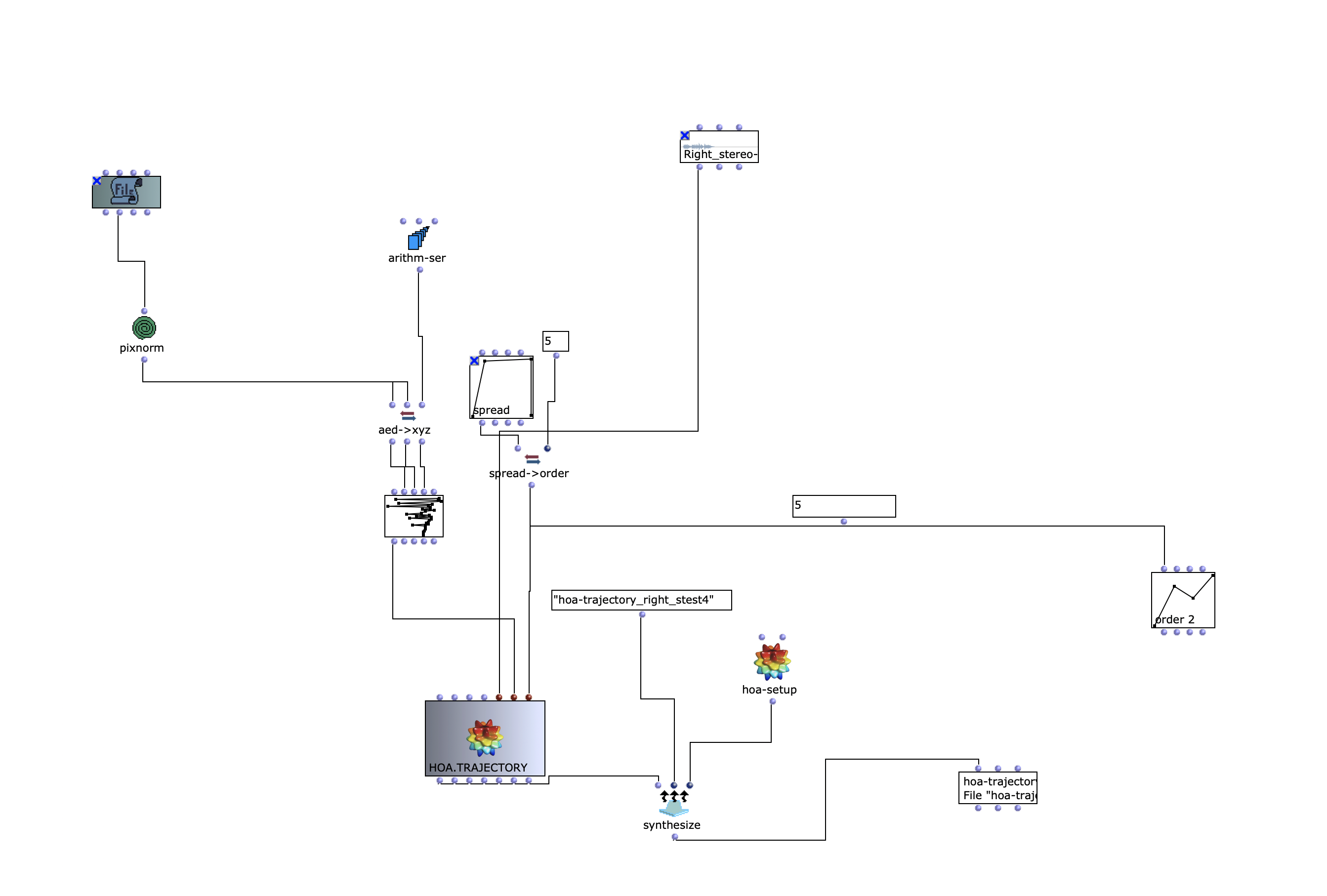
Once all the graphics of the picture object have been read out, they must be divided into rectangles and circles for further processing. If only one rectangle is found, the position and dimension of the rectangle and the two specifications for the length and number of loudspeaker arrays can first be used to determine the position of each individual loudspeaker within the array in meters. If there are several rectangles, this step is not necessary and the center points of all specified rectangles are simply determined. It is then possible to calculate the Euclidean distance from all sources to each individual loudspeaker on the same scale using another Lisp function. It should be noted that all graphics drawn by the user in the Picture object that do not correspond to a rectangle or a circle are ignored and not taken into account for the further calculations. As any number of virtual sound sources can be specified for the application, all circles that exist in the picture object are also captured in this step, whereby the order is irrelevant.
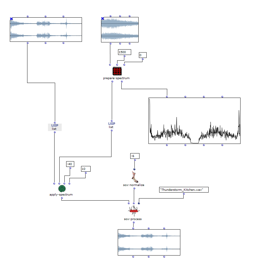
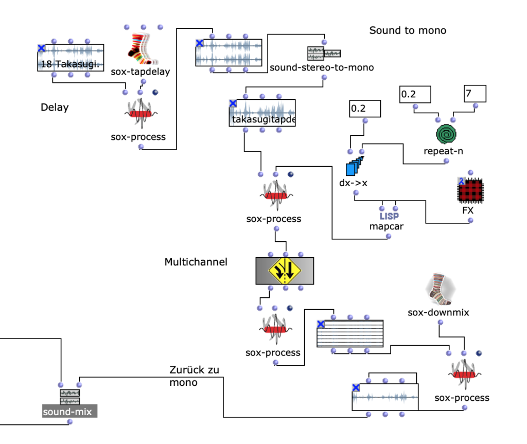
Sound processing
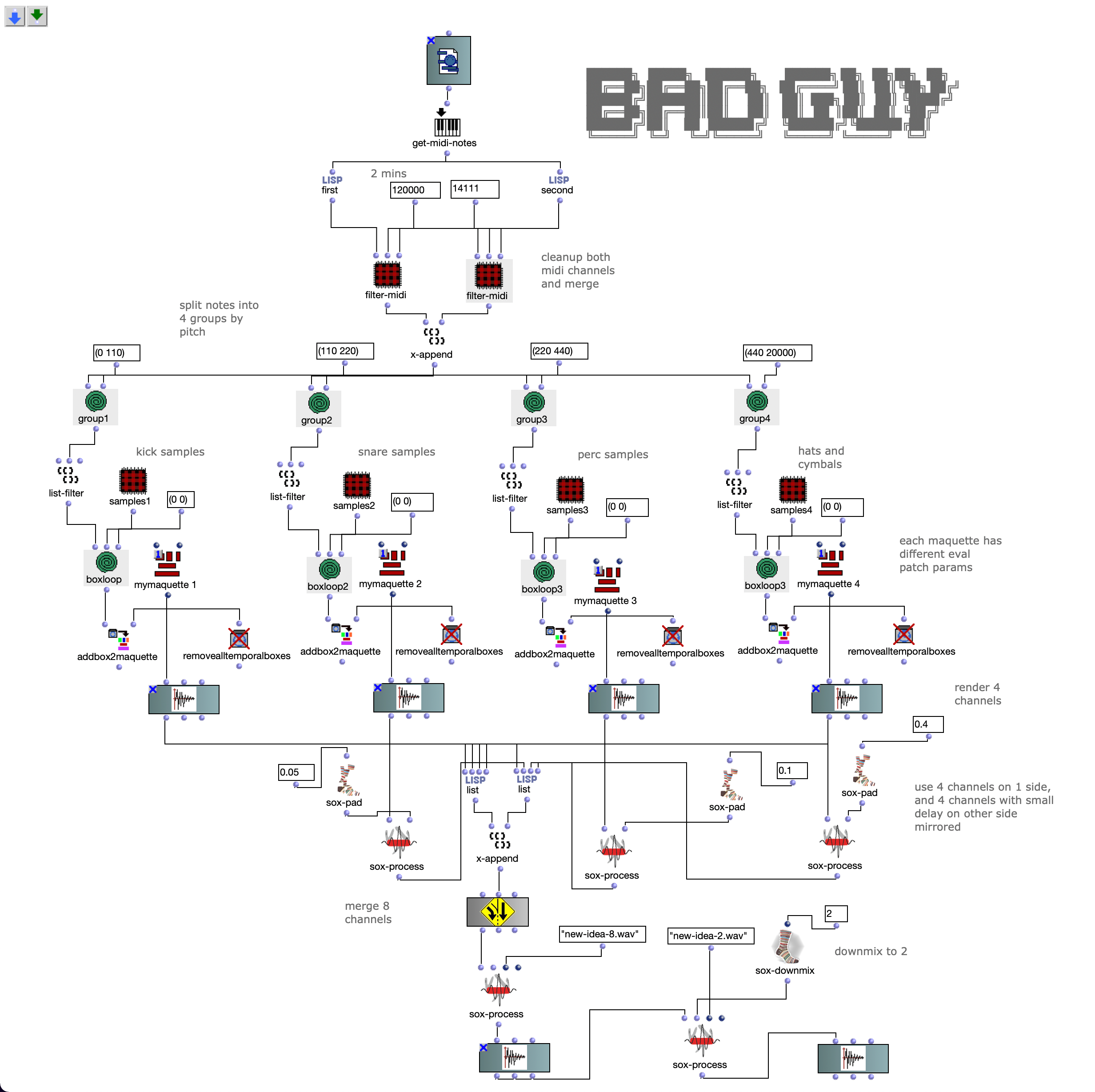
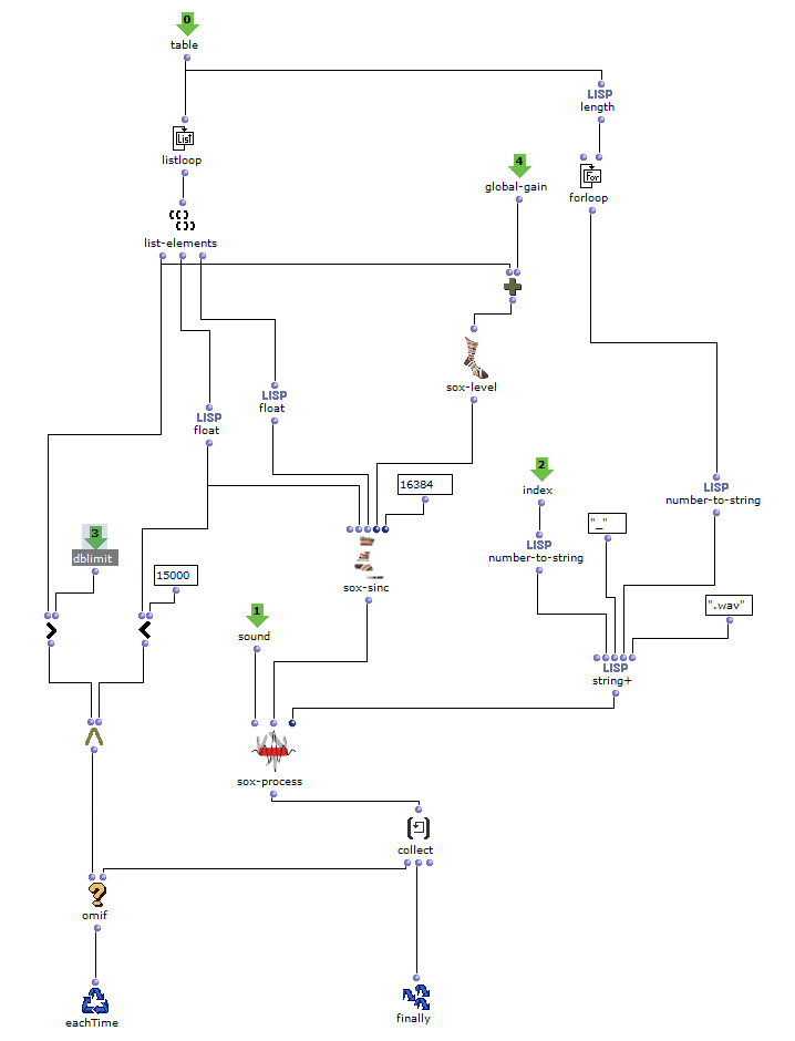
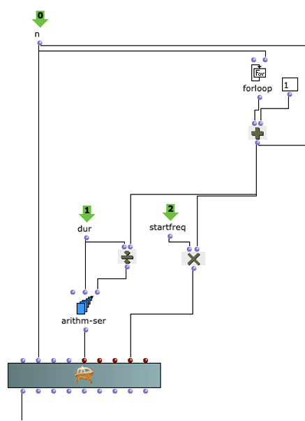
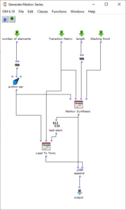
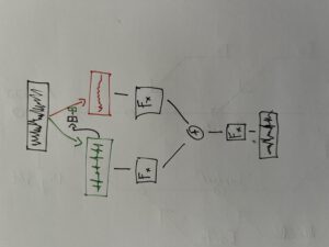
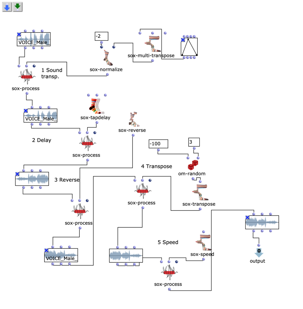
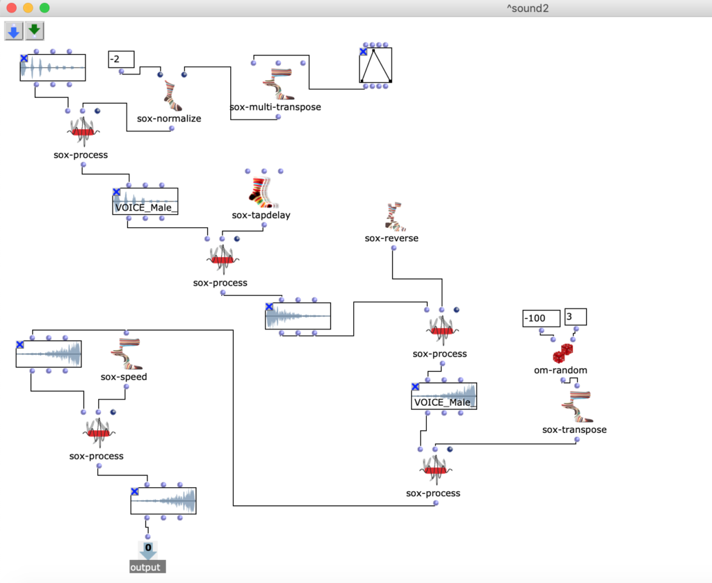
Sound processing is implemented in the next section of the program. Basically, a multi-channel file is created with the sound file specified by the user together with the previously calculated distances, which can be used for the intended loudspeaker array. This process takes place in a nested OM loop with two levels.
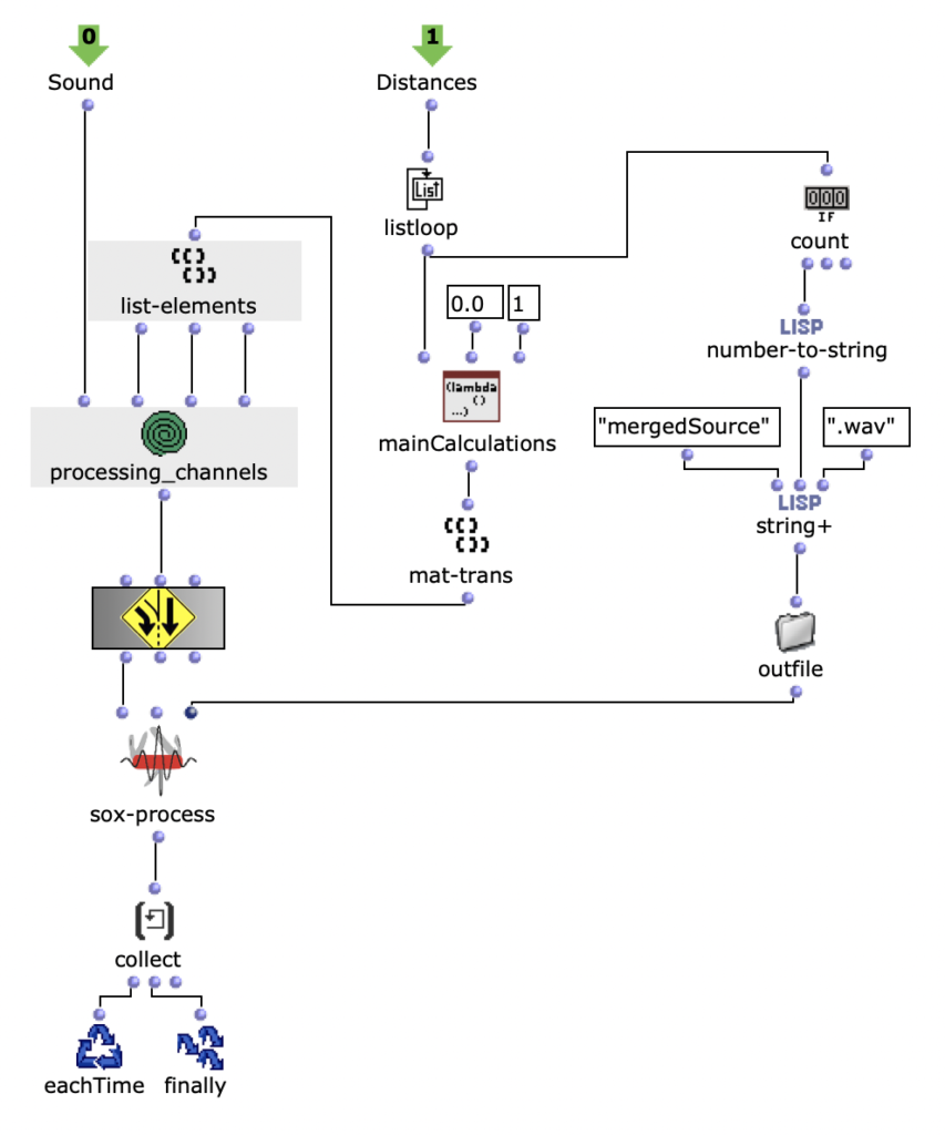
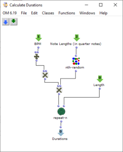
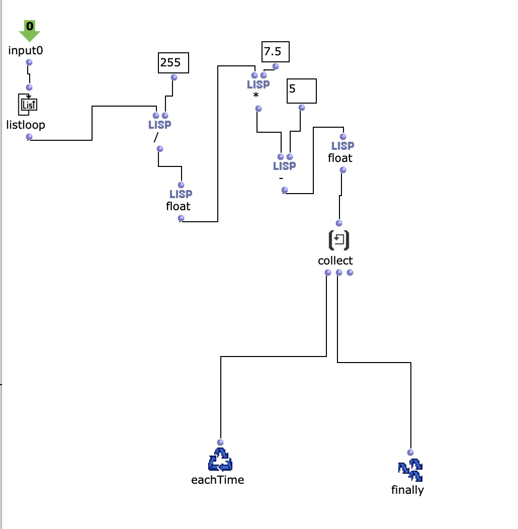
In the first level, it is first iterated over each element within the distance list. Each of these elements corresponds to a list that belongs to a virtual sound source, which contains the distances to each loudspeaker. Before the process enters the second level of the loop, further calculations are performed in a Lisp function using the current distance list.
This function iterates over each distance and determines the time delay, volume reduction and a cutoff frequency for a lowpass filter to calculate the air absorption of high frequencies and collects them in a list. In the next step, the result of this Lisp function is used to enter the second level of the loop.
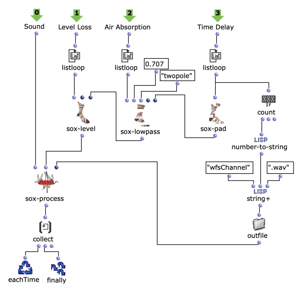
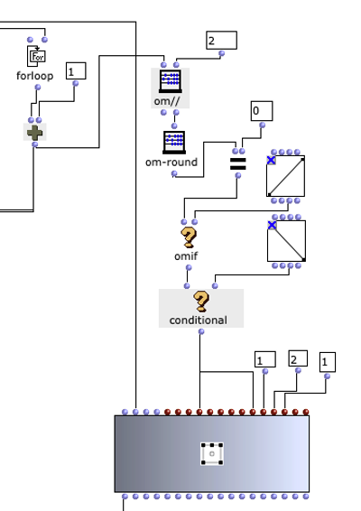
Here, the respective SoX effect is applied to the calculated value; SoX level for volume reduction, SoX lowpass for air absorption and SoX pad for the time delay. The resulting audio file is saved for each iteration. Each of the three lists has as many values as the previously calculated distances from the current sound source to the speakers. This means that each audio file saved in this loop represents one channel of the subsequent multi-channel file for the current sound source.
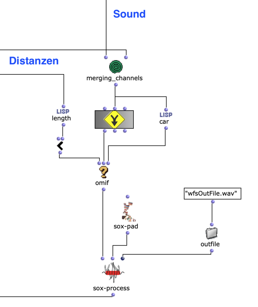
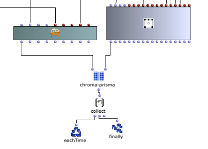
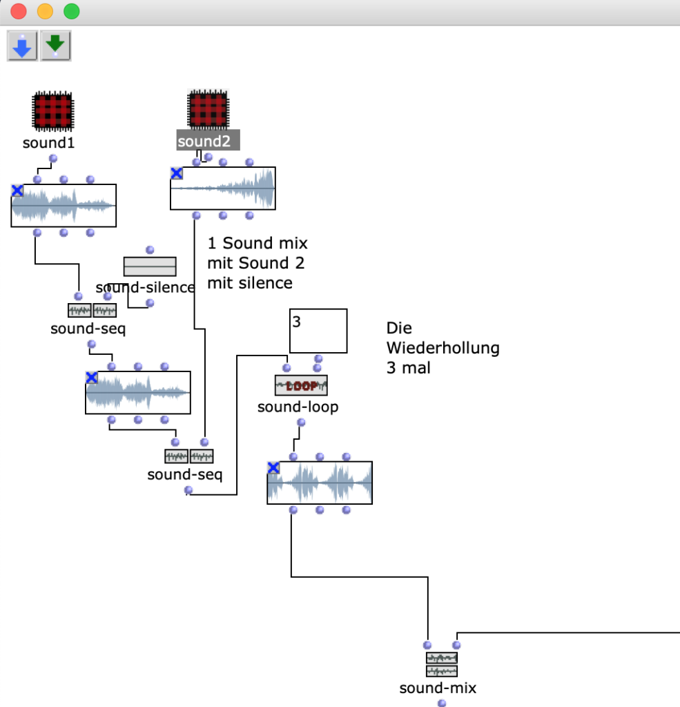
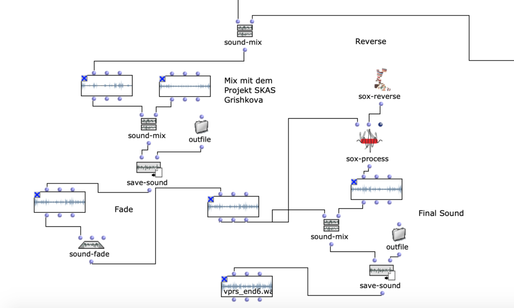
The multi-channel file can now be created in the next step in the first layer with SoX-Merge and stored temporarily at the end of the loop. This process is repeated for all remaining virtual sound sources (if existing) and are collected as the output of this upper loop. All multi-channel files of the respective sound sources are then merged with a SoX-Mix.
If only one virtual sound source is specified by the user, the output of the outermost loop will only consist of a single multi-channel file for this one source. In this case, the SoX-Mix is not required and it would even lead to an error during the evaluation of the program if the input of the SoX-Mix consisted of only one audio file. The OM-If therefore avoids the use of the SoX-Mix as soon as the output of the patcher, in which the distances are determined, only consists of one list, which means that only one circle for a virtual sound source has been drawn in the picture object.
Finally, silence can be added to the multi-channel file using the SoX pad, depending on preference, if the selected audio file is particularly short, for example. At the same time, the final multi-channel file is saved in Outfile as “wfsOutFile.wav”.


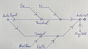
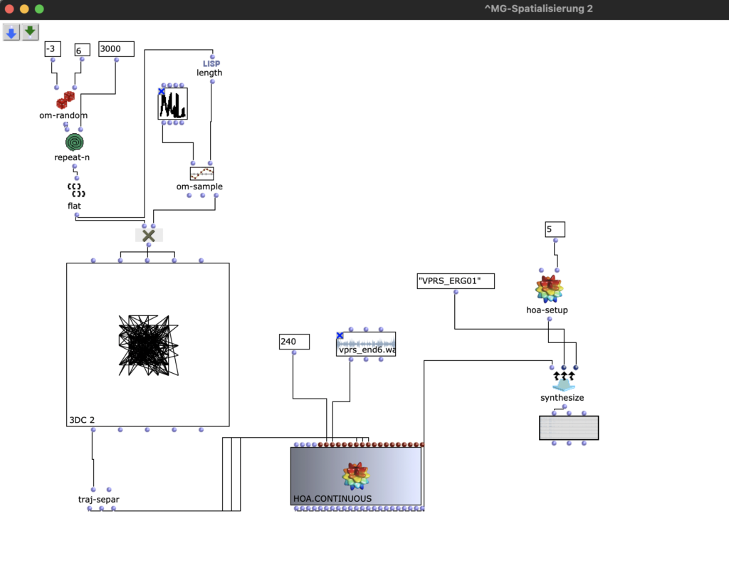
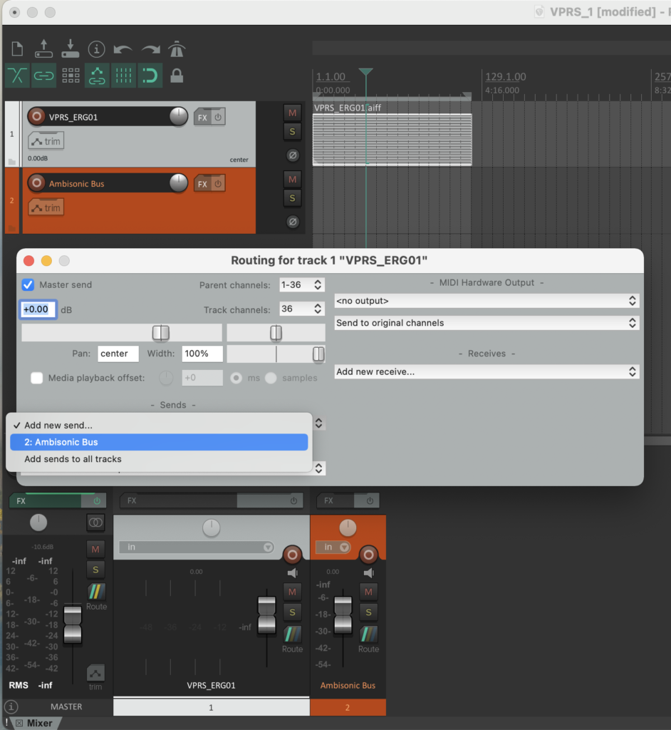
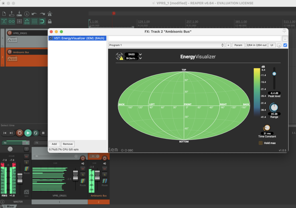
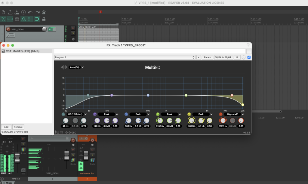
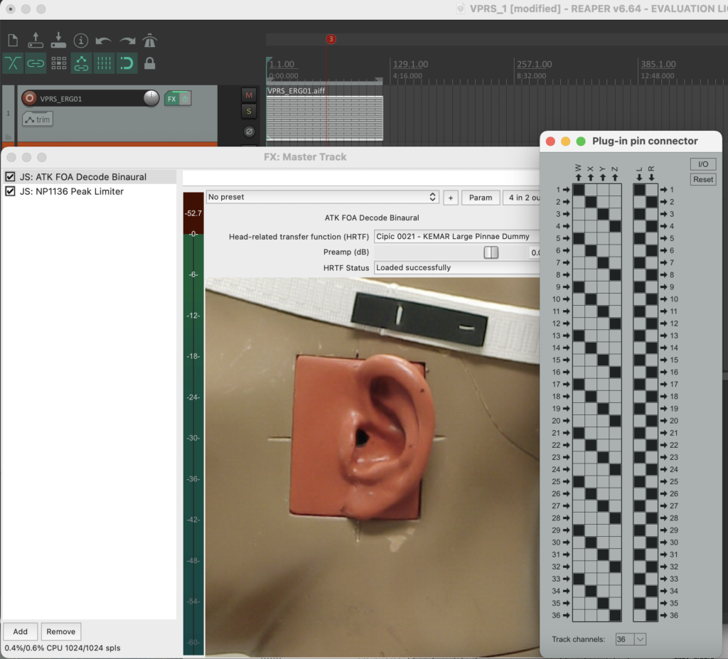
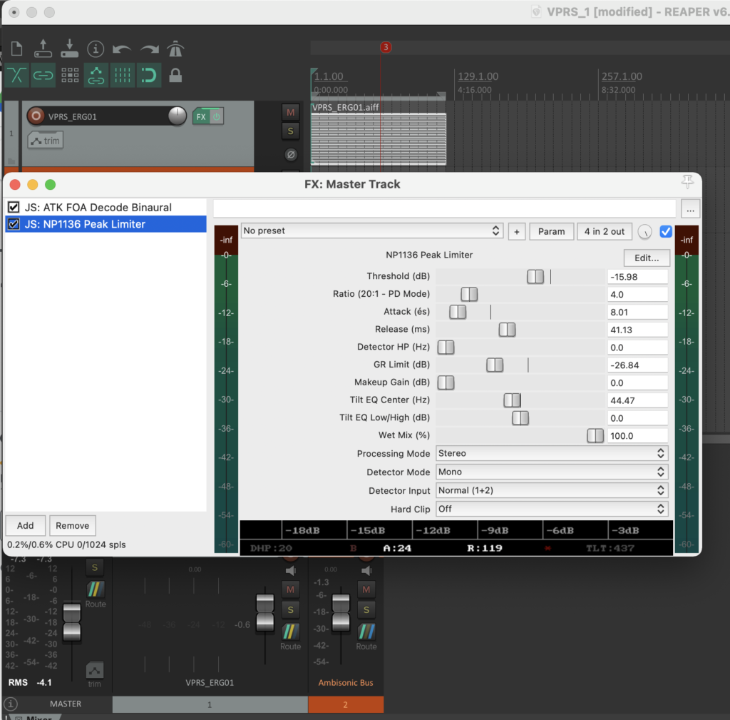
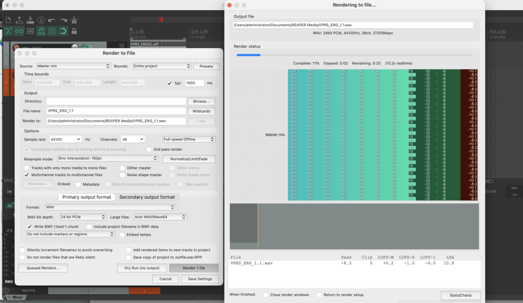

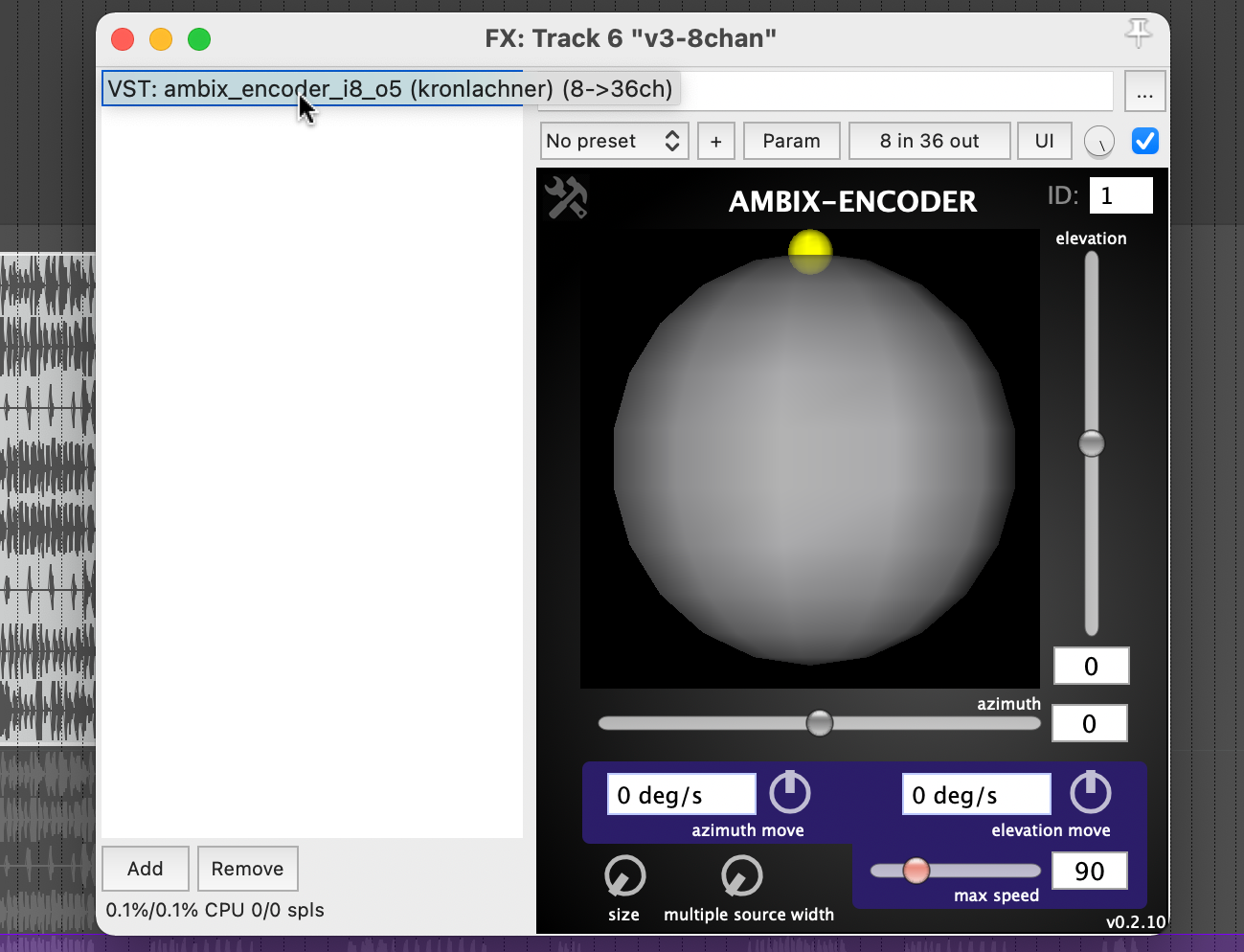
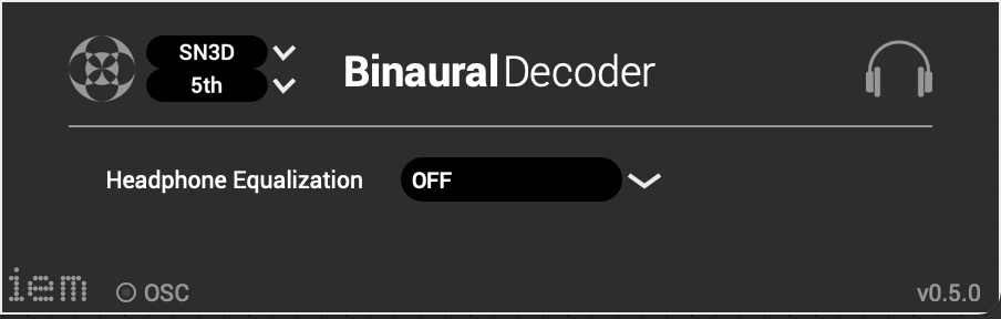
 The stereo and mono files were first encoded in 5th order Ambisonics (36 channels) and then converted into two channels using the binaural encoder.
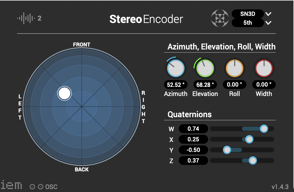
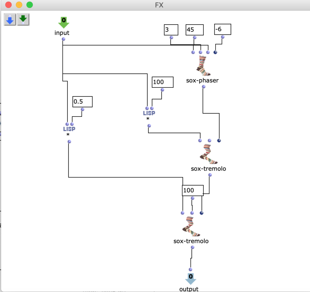
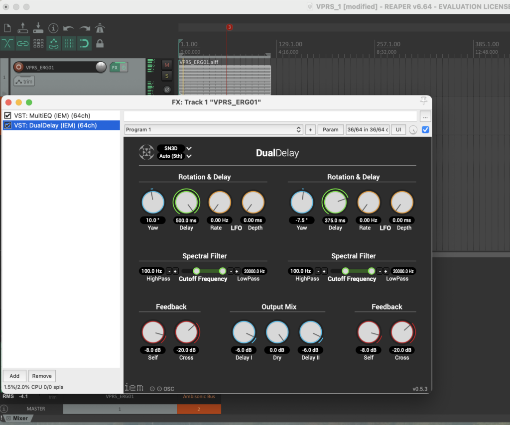
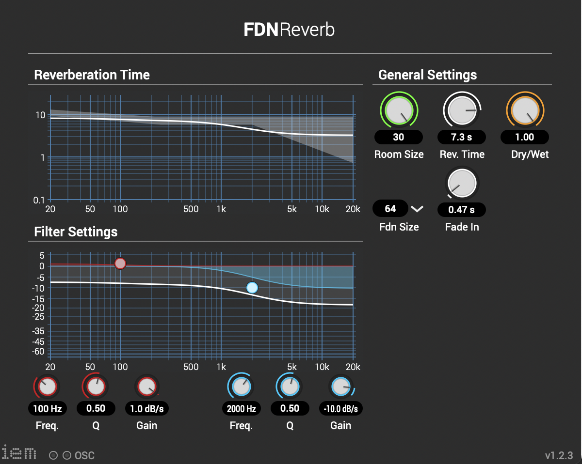
 Other post-processing effects (Detune, Reverb) were programmed by myself and are available on Github. The reverb is based on a paper by James A. Moorer About this Reverberation Business from 1979 and was written in C. The algorithm of the detuner was written in C from the HTML version of Miller Puckette’s handbook “The Theory and Technique of Electronic Music”. The result of the last iteration can be heard here.