Common Lisp, Computer-aided Composition, OM-SoX, OpenMusic, Sonification

Sonification of Image Sequences

Abstract: This project deals with the design of an OpenMusic application that has the goal of converting image sequences into a symbolic music representation consisting of three voices.

Responsible: Mads Clasen

Source material and preparation

The image sequence can be individual frames from a video, a series of images from an artist or images you have compiled yourself. These must first be available in a folder on the relevant computer. If it is a video, it must first be broken down into its frames outside of OpenMusic. In Python, this can be done very easily in just a few lines with the help of the OpenCV library.

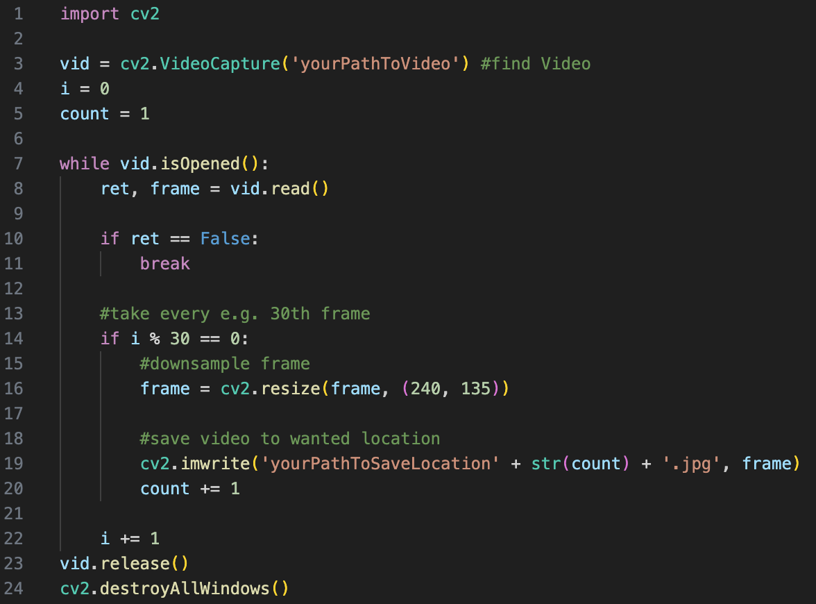
Fig. 1: Splitting video in Python

As can be seen in the code example, the resulting images should also be named numerically with numbers from 1 to n and, depending on the computing power of the computer and the number of images, be downsampled. This, as well as the installation of the Pixels Library in OpenMusic itself, is necessary for the patch to work properly.

Sonification

Note values

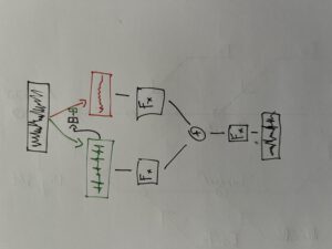
After specifying the file path, file format and number of images, the desired images are loaded into a picture-lib object and summarised as a list. The average R, G and B colour value is read from each image in this list and mapped to a corresponding note. In this case, the R, G and B values are treated as different voices and each have their own note range within which they move. This range is additionally subdivided into microtonal steps (1/8 notes) to which the values are finally mapped. A value of 1 corresponds to the highest possible note and 0 to the lowest. Accordingly, one note for each of the three voices is read from an image.

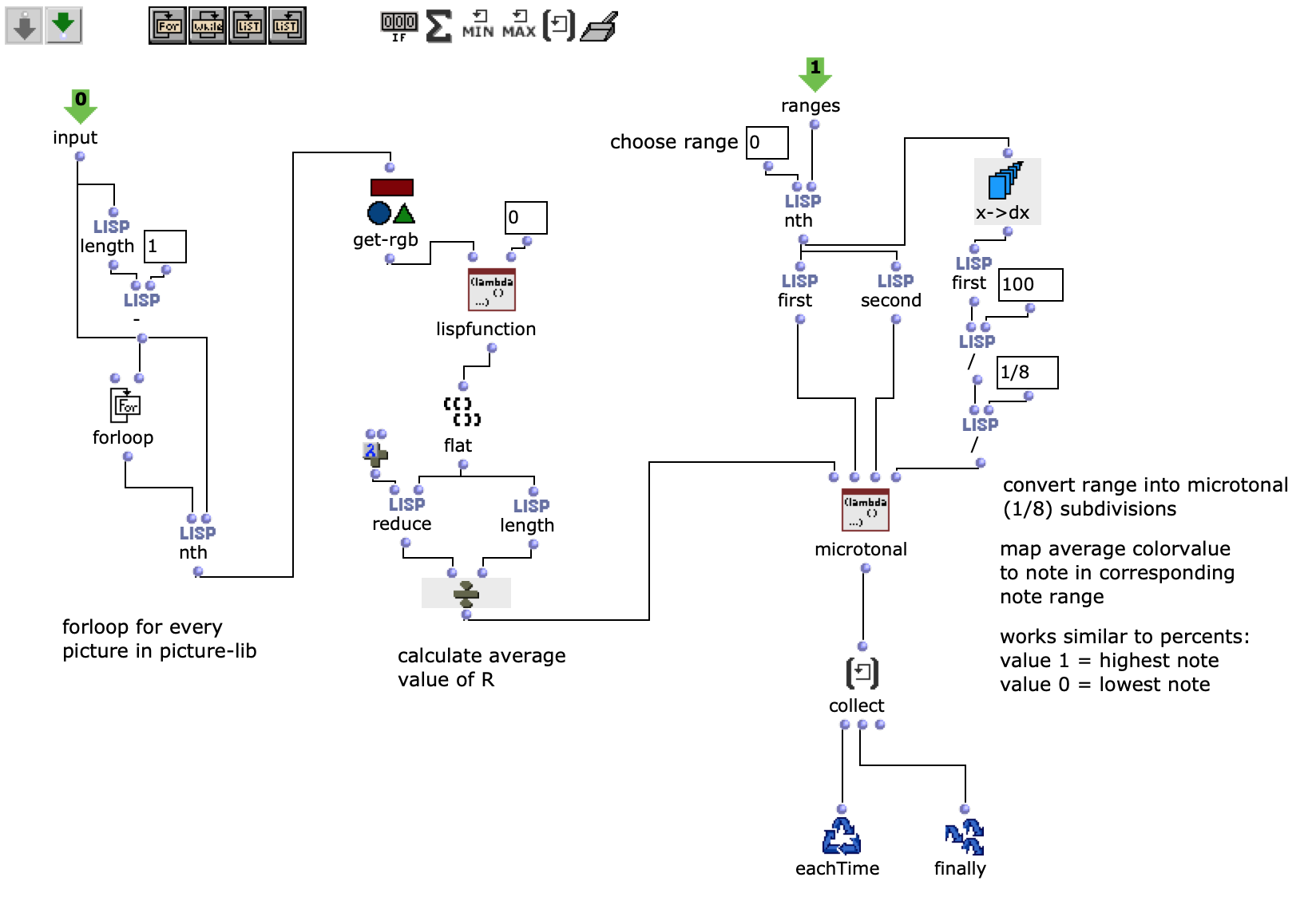
Fig. 2: Generation of a score line

The note ranges in which the colour values move can be adjusted using the corresponding chord objects; it is also possible to transpose all ranks uniformly by a desired value in midicents. The preset values correspond to the approximate note ranges of soprano (R), alto (G) and bass (B) voices. After running through the entire image sequence, there are now three voices with a number of notes corresponding to the number of images entered. These voices are processed independently of each other in the next step.

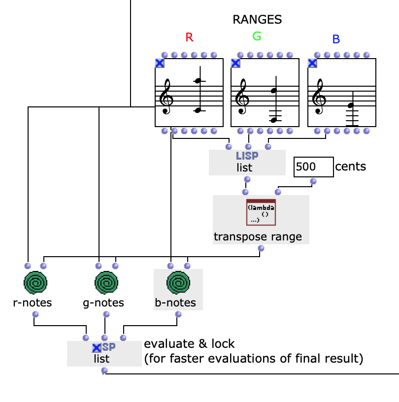
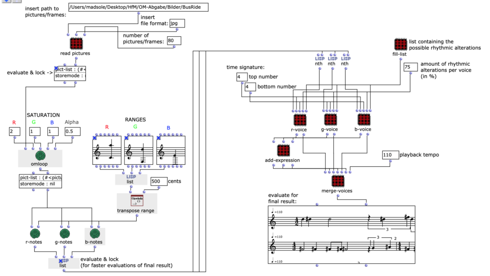
Fig. 3: Mapping the RGB values onto note values

Rhythm

As I have decided to use voice objects because of the direct way of influencing rhythm, the rhythm trees required for this are created first. Or rather the two building blocks of a rhythm tree : time signature and proportions. A list is created for each of these, based on the number of notes and the time signature, which are later merged into the required rhythm tree form using a simple mat-trans object.

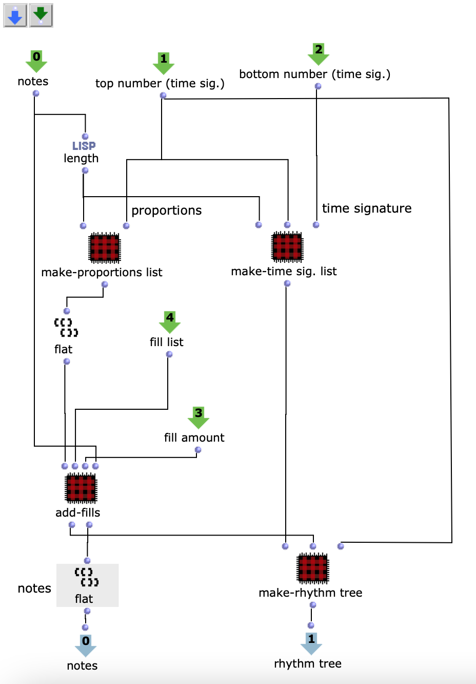
Fig. 4: Generating the rhythm tree

Before this, however, the list responsible for the proportions is enriched with ostinato. For this purpose, there is a second list containing various possibilities for such ostinato, from which one is selected at random and placed in a random position in the proportion list. As this increases the number of note values, new notes corresponding to the embellishment are inserted at the same position in the list containing the notes. Starting from the original note, a decision is made between constant, ascending or descending notes. The strength with which these ornaments are to be included in the parts can also be adjusted.

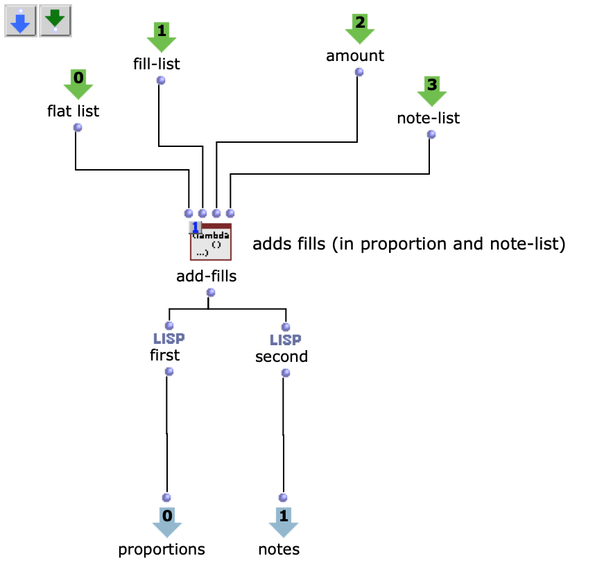
Fig. 5: Addition of rhythmic ornaments

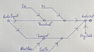
Dynamics

The edited proportions are then merged with the list that determines the time signature to form the rhythm tree . The corresponding note list goes through one more step, in which a random velocity value is assigned to each note.

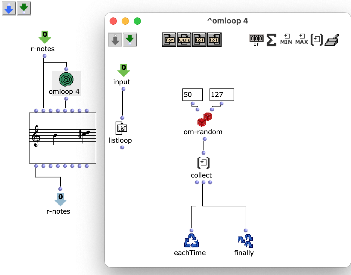
Fig. 6: Creating dynamics

Finally, the note lists are combined with their respective rhythm tree in a voice object to form a voice, resulting in a total of three voices (R, G, B), which can then be combined in a poly object.

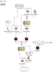
Image processing

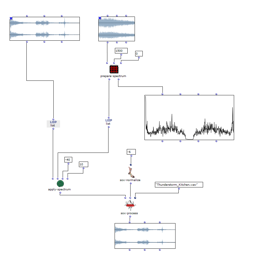
In order to additionally influence the sound result, it is possible to edit the saturation of the colour values of individual images of the selected sequence. The original images are then mixed with the altered ones.

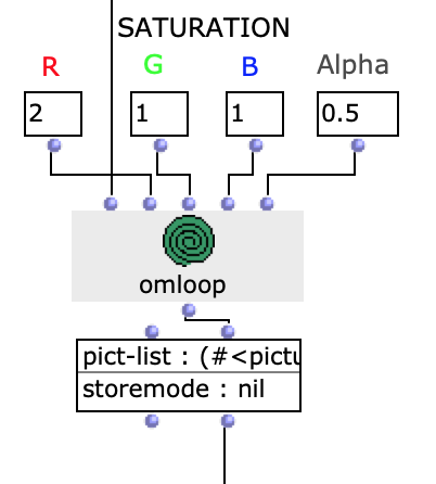
Fig. 7: Changing colour values

Example

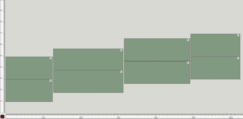
In the following, the frames of a video taken during a bus journey and showing the surroundings were used as the image sequence. Every thirtieth frame was saved. In the patch, the option of colour manipulation was also used to make the sequence a little more varied.

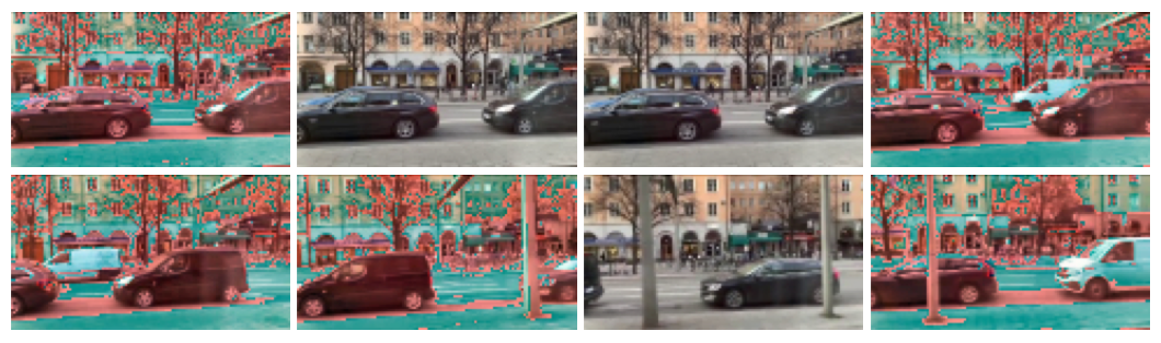
Fig. 8: Edited image sequence

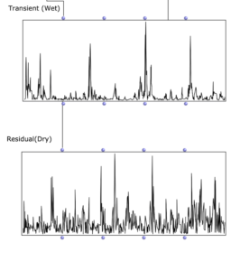
After evaluating the remaining patch, a possible end result of this image sequence could look and sound as follows:

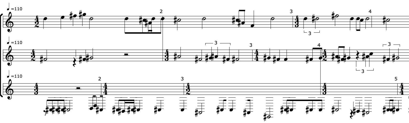
Fig. 9: Excerpt of symbolic representation

ByAlexander Nguyen

Common Lisp, Digital Signal Processing, OM-SoX, OpenMusic

HOA Encoder using OM-SoX

Abstract: OpenMusic and the OM-SoX library were used to create a way to encode mono audio files as a 3D Ambisonics signal up to the third order.

Responsible: Alexander Nguyen (WS 2023/24)

Main text:

Ambisonics

Ambisonics is a method for describing a two- or three-dimensional sound field (in the following I shall restrict myself to 3D Ambisonics). Ambisonics uses a basis of orthogonal functions and the spherical coordinate system to describe the sound field along a spherical surface resulting from a sound source . The simplest case is “Zero-th Order Ambisonics”, which resembles an ideal omnidirectional microphone: exactly one audio channel is used (also called the “W” channel, according to Furse-Malham naming). With “First Order Ambisonics” (FOA), the signal is split into an additional three channels (three bases): These are the three “directional” components (also called X, Y, Z channels). Assuming an ideal point sound source is placed at the end of one of these axes, then only this axis (with respect to the same ordinal number) will contain the signal. In the case of Ambisonics, the channels of lower orders are always included, i.e. the FOA signal consists of a total of four audio channels. In general, the number of channels for a 3D Ambisonics signal of the $n$th order can be calculated using the formula $(n+1)^2$ (i.e. for $n=0$: 1; for $n=1$: 4, for $n=2$: 9, for $n=3$: 16). Ambisonics signals with ‘higher’ order numbers (…, 2, 3, 4, …) are also referred to as Higher Order Ambisonics (HOA).

Channel Numbering

An HOA signal therefore consists of several components. There are several approaches to sorting the components in a multi-channel audio file. The sorting chosen here for this project is “Ambisonic Channel Numbering” (ACN), in which each channel is assigned an integer number starting at zero (0). The first channel is therefore labeled “0”, the second channel “1”, the third channel “2” and so on. This numerical designation can be used to determine the ‘order’ ($l$) and the ‘degree‘ ($m$) to which the component belongs. See Table 1 for an overview of all components of 3rd Order Ambisonics (3OA) – and a collation with an alternative labeling, “Furse Malham” (FuMa).

Auswertung der Formeln für l und m anhand der ACN-Werte. Zusätzlich die alternative Bezeichnung nach Furse-Malham (FuMa).

Table 1. Evaluation of the formulas for l and m based on the ACN values. In addition, the alternative designation according to Furse-Malham (FuMa)

Normalization

The values $l$ (order) and $m$ (degree) are used to calculate a normalization factor for each audio channel. The normalization used here is called “Semi-Normalized 3D” (SN3D). See Table 2 for an overview of the normalization factors for all components of 3rd Order Ambisonics.

ACN together with SN3D normalization reflect a currently common convention called ambiX (Nachbar et al., 2011).

SN3D-Faktoren für Order l und Degree m, d.h. N_lm^((SN3D)). Hinweis: Wenn also m=0 ist, ist auch immer N_l0^((SN3D) )=1, und die Tabelle ist symmetrisch bezüglich m.

Table 2. SN3D factors for order $l$ and degree $m$, i.e. $N_{lm}^{(SN3D)}$. Note: If $m=0$, then $N_{l0}^{(SN3D)}=1$, and that the table is symmetric with respect to $±m$.

Encoding

To map a point sound source in Ambisonics, its audio signal is added to each of the audio channels, weighted using the normalization factor just described and an attenuation factor. The attenuation factor, which will be defined below, depends on the angle of incidence (described in the spherical coordinate system) and the ACN number (i.e. order and degree). An intuition (w.r.t. FOA): The attenuation is minimum (0 dB or multiplication factor 1, respectively) if the angle of incidence coincides with one of the axes in an ordinary 3-dimensional coordinate system ($x$, $y$ or $z$), maximum (-∞ dB or factor 0) if it is perpendicular to it.

In Ambisonics, the 3D coordinate system is usually defined as follows: The “front” (relative to the listener’s point of view) is defined as the positive x-axis. Being a right-handed system, this implies that the positive y-axis points to the “left” and the positive z-axis points “up“. For the transformation to polar coordinates, i.e. to the spherical coordinate system, one defines 0° azimuth (θ) coincident to the positive x-axis on the xy-plane, counterclockwise. 0° elevation (ϕ) coincident to the xy-plane, maximum positive, if coincident to the positive z-axis (see Figure 1), with:

$0≤θ≤2π$

$-π/2≤ϕ≤π/2$

Abbildung 1. Visualisierung des Koordinatensystems und der Bezugspunkte. Positiv-x = vorne, positiv-y = links, positiv-z = oben. θ (theta) linksdrehend (0° = vorne), ϕ „aufwärtsdrehend“ (0° = in der xy-Ebene).

Figure 1. Visualization of the coordinate system and the reference points. Positive-x = front, positive-y = left, positive-z = top. θ (theta) left-turning (0° = front), ϕ “up-turning” (0° = in the xy plane).

In order to encode a time $t$-dependent signal $S(t)$ of a point sound source with angles of incidence $θ, ϕ$ in Ambisonics, the eventual Ambisonics signal component is calculated separately for each channel $B_l^m$. To do this, the signal is multiplied by the attenuation factor $Y_l^m$ :

$B_l^m (t) := S(t)\cdot Y_l^m (\theta, \phi)$

The formula for the attenuation factor is (see Nachbar et al., 2011):

\[
Y_l^m(\theta, \phi) :=N_l^{|m|} \cdot P_l^{|m|}(sin(\phi)) \cdot \begin{cases}
sin(|m|\theta) & \text{if } m < 0\\
cos(|m|\theta) & \text{if } m > 0\\
1 & \text{if } m=0
\end{cases}
\]

where $P_l^m$ is the “associated Legendre polynomial” of $l$-th order and $m$-th degree, and $P_l$ is the (unassociated) Legendre polynomial of $l$-th order (in the Rodrigues representation). These are defined as follows:

\[\begin{eqnarray*}
P_l(x) &:=& \frac{1}{2^l\cdot l!}\cdot \frac{d^l}{dx^l} \left[ (x^2-1)^l \right] \\
P_l^m(x) &:=& (1-x^2)^{\frac{m}{2}}\cdot \frac{d^m}{dx^m} \left[ P_l(x) \right] \\
&=& \frac{1}{2^l\cdot l!}\cdot (1-x^2)^\frac{m}{2}\cdot\frac{d^{l+m}}{dx^{l+m}} \left[ (x^2-1)^l \right]
\end{eqnarray*}\]

For example:

\[\begin{eqnarray*}
P_0^0(x) &=& (1-x^2)^\frac{0}{2}\cdot \frac{d^0}{dx^0} \left[ P_0(x) \right] \\
&=& 1\cdot P_0(x) = 1 \cdot 1 = 1
\end{eqnarray*}\]

\[\begin{align*}
P_2^1(x) &= (1-x^2)^\frac{1}{2}\cdot \frac{d^1}{dx^1} \left[ P_2(x) \right] \\
&= (1-x^2)^\frac{1}{2}\cdot \frac{d}{dx} \left[ \frac{1}{2^2\cdot 2!}\cdot \frac{d^2}{dx^2} [ (x^2-1)^2 ] \right] \\
&= (1-x^2)^\frac{1}{2}\cdot \frac{d}{dx} \left[ \frac{1}{8}\cdot \frac{d^2}{dx^2} [ x^4-2x^2+1 ] \right] \\
&= (1-x^2)^\frac{1}{2}\cdot \frac{d}{dx} \left[ \frac{1}{8}\cdot \frac{d}{dx} [ 4x^3-4x ] \right] \\
&= (1-x^2)^\frac{1}{2}\cdot \frac{d}{dx} \left[ \frac{1}{8}\cdot [ 12x^2-4 ] \right] \\
&= (1-x^2)^\frac{1}{2}\cdot \frac{d}{dx} \left[ \frac{3}{2} x^2 -\frac{1}{2} \right] \\
&= (1-x^2)^\frac{1}{2}\cdot \left[ \frac{3\cdot 2}{2} x \right] \\
&= (1-x^2)^\frac{1}{2}\cdot \frac{6}{2}x \\
&= 3x\cdot (1-x^2)^\frac{1}{2} \\
\end{align*}\]

Let $x≡sin(ϕ)$, then we obtain one of the spherical harmonics (see Table 3 for further examples):

\[\begin{align*}
P_2^1(sin(\theta)) &= 3\cdot sin(\phi)\cdot \sqrt{1-sin^2(\phi)} \\
&= 3\cdot sin(\phi)\cdot \sqrt{cos^2(\phi)} \\
&= 3\cdot sin(\phi)\cdot cos(\phi) \\
&= \frac{3\cdot sin(2\phi)}{2} \\
\end{align*}\]

The formulas for FOA are thus:

\[\begin{align*}
\text{ACN 1 / W:}\qquad &B_0^0(t) =S(t)\cdot Y_0^0(\theta, \phi)= S(t) \\
\text{ACN 2 / Y:}\qquad &B_1^{-1}(t) =S(t)\cdot Y_1^{-1}(\theta, \phi)= S(t)\cdot cos(\phi) \cdot sin(\theta) \\
\text{ACN 3 / Z:}\qquad &B_1^0(t) =S(t)\cdot Y_1^1(\theta, \phi)= S(t)\cdot sin(\phi) \\
\text{ACN 4 / X:}\qquad &B_1^1(t) =S(t)\cdot Y_1^1(\theta, \phi)= S(t) \cdot cos(\phi) \cdot cos(\theta) \\
\end{align*}\]

Tabelle 3. Ambisonics-Formeln bis zur dritten Ordnung (ACN-Zählung, SN3D-Normalisierung, 0≤θ≤2π Azimut (0° = vorne, linksdrehend), -π/2≤ϕ≤π/2 Elevation (0° = auf der xy-Ebene, aufwärtsdrehend)).

Table 3. Ambisonics formulas up to third order (ACN counting, SN3D normalization, $0≤θ≤2π$ azimuth (0° = forward, counterclockwise), $-π/2≤ϕ≤π/2$ elevation (0° = on the xy plane, upward rotation))

ByLukas Körfer

Common Lisp, OM-SoX, OpenMusic, Wellenfeldsynthese

Wave field synthesis with OM-SoX

Abstract: This final project was created at the end of the winter semester 2023/24 as part of the course “Symbolische Klangverarbeitung und Analyse/Synthese” (eng. Symbolic Sound Processing and Analysis/Synthesis) of the MA Music Informatics. An application for sound spatialization was developed in the program OpenMusic using the library OM-SoX implementing Steinberg and Snow’s “acoustic curtain”, a technique for wave field synthesis.

Responsible: Lukas Körfer

Wave field synthesis

Wave field synthesis (WFS for short) is the spatialization of virtual sound sources using a high-density loudspeaker array. This spatialization technique attempts to reproduce a physical soundfield over an extended area in a way to provide for multiple non-conicident listening positions a congruent impression of the localization of sound sources. This is achieved by generating a wave field consisting of a large number of individual sound sources that are synchronized in such a way that a coherent sound wave is created, for which given certain constraints it should be possible to localize a virtual sound source in the room.

For a better understanding of how WFS works, the subject can be approached via the physical phenomenon of interference pattern formation behind an obstacle with openings. When a wave encounters one or more slits, it is diffracted through the openings and propagates behind the obstacle. This leads to the formation of a pattern of wave interference on the other side of the obstacle. Similarly, wave field synthesis uses an array of loudspeakers to generate a coherent sound wave. This requires precise calculation and control of the phase and amplitude relationships of the sound waves emanating from each speaker. These calculations are dependent on the distances of each individual loudspeaker in the array relative to the position in space of the respective virtual sound source.

Project description

For this project, a program was to be created with the general goal of ultimately obtaining a multi-channel audio file that can be used for wave field synthesis with a loudspeaker array through certain influence and adjustments by a user. To achieve this, it was first necessary to design which parameters should be set and influenced by the user of the program.

User input

In addition to the audio file, which is to be used for spatialization, the user must specify certain information about the loudspeaker array on the one hand and the position or positions of one or more virtual sound sources relative to the loudspeaker array on the other. In order to make the configuration of the program as simple and intuitive as possible, I have decided to mainly use a picture object in which the structure can be recorded. The positions of the loudspeakers can be specified by drawing a rectangle and those of the virtual sound sources with circles. One or more circles can be drawn, with each circle representing a sound source. The loudspeakers can be specified in two different ways. If only a single rectangle is drawn in the picture object, this represents the area of a loudspeaker array. In order to be able to determine the specific positions of the individual loudspeakers in the next step of the program, two additional pieces of information are required. Firstly, the length of the loudspeaker array in meters; this also influences the scale for the complete drawn setup. Secondly, the number of loudspeakers in the drawn area must be specified. As soon as more than one rectangle is specified by the user, each individual rectangle represents an individual loudspeaker. In order to be able to specify a scale for the drawn structure in this variant – which was previously possible by specifying the length of the loudspeaker array – the width/height of the area of the complete picture object can now be specified. The first variant, where the loudspeaker array can only be drawn with a rectangle, makes the application much less complicated, but also requires the loudspeakers to be linear and evenly spaced.

Calculating distances

Once all the graphics of the picture object have been read out, they must be divided into rectangles and circles for further processing. If only one rectangle is found, the position and dimension of the rectangle and the two specifications for the length and number of loudspeaker arrays can first be used to determine the position of each individual loudspeaker within the array in meters. If there are several rectangles, this step is not necessary and the center points of all specified rectangles are simply determined. It is then possible to calculate the Euclidean distance from all sources to each individual loudspeaker on the same scale using another Lisp function. It should be noted that all graphics drawn by the user in the Picture object that do not correspond to a rectangle or a circle are ignored and not taken into account for the further calculations. As any number of virtual sound sources can be specified for the application, all circles that exist in the picture object are also captured in this step, whereby the order is irrelevant.

Sound processing

Sound processing is implemented in the next section of the program. Basically, a multi-channel file is created with the sound file specified by the user together with the previously calculated distances, which can be used for the intended loudspeaker array. This process takes place in a nested OM loop with two levels.

In the first level, it is first iterated over each element within the distance list. Each of these elements corresponds to a list that belongs to a virtual sound source, which contains the distances to each loudspeaker. Before the process enters the second level of the loop, further calculations are performed in a Lisp function using the current distance list.

This function iterates over each distance and determines the time delay, volume reduction and a cutoff frequency for a lowpass filter to calculate the air absorption of high frequencies and collects them in a list. In the next step, the result of this Lisp function is used to enter the second level of the loop.

Here, the respective SoX effect is applied to the calculated value; SoX level for volume reduction, SoX lowpass for air absorption and SoX pad for the time delay. The resulting audio file is saved for each iteration. Each of the three lists has as many values as the previously calculated distances from the current sound source to the speakers. This means that each audio file saved in this loop represents one channel of the subsequent multi-channel file for the current sound source.

The multi-channel file can now be created in the next step in the first layer with SoX-Merge and stored temporarily at the end of the loop. This process is repeated for all remaining virtual sound sources (if existing) and are collected as the output of this upper loop. All multi-channel files of the respective sound sources are then merged with a SoX-Mix.

If only one virtual sound source is specified by the user, the output of the outermost loop will only consist of a single multi-channel file for this one source. In this case, the SoX-Mix is not required and it would even lead to an error during the evaluation of the program if the input of the SoX-Mix consisted of only one audio file. The OM-If therefore avoids the use of the SoX-Mix as soon as the output of the patcher, in which the distances are determined, only consists of one list, which means that only one circle for a virtual sound source has been drawn in the picture object.

Finally, silence can be added to the multi-channel file using the SoX pad, depending on preference, if the selected audio file is particularly short, for example. At the same time, the final multi-channel file is saved in Outfile as “wfsOutFile.wav”.

Video

This video shows how a multi-channel file with 16 channels, which was previously created in OpenMusic (left), is played with the Binauralix programme (right). In Binauralix, the sources representing the speakers are arranged as a speaker array according to the settings in the OM patch. The position of the listener relative to this array influences the synthesis of the stereo signal that can be heard in the video.

ByFlorian Simon

OM-SoX, OpenMusic

Interspaces – Acousmatic study with OM-SoX

Interspaces juxtaposes sounds from human civilization with sounds from nature. Four pairs of field recordings are presented, which are filtered according to the principle of a vocoder according to the spectrum of a section of the counterpart.

Responsible: Florian Simon

Interspaces shows the following four pairs (format: total recording – source of the spectrum):

Chirping Arctic terns – Vowel “E” called by humans
Lively market, people talking and calling – Arctic tern call
Rippling of a river – Accelerating car
Main road – rushing of a river
Forest scenery, rustling leaves and birds – Train horn
Station concourse – chirping of a songbird
Thunderstorm – clinking of cutlery
Business in a restaurant kitchen – thunder

The field recordings come from the FreeToUseSounds library.

Interspaces uses an equilateral octagonal loudspeaker arrangement, whereby the two channels of the source material are each placed at opposite points in the array. The two recordings of a pair are also offset by 90 degrees from each other by default, so that four sound sources can be perceived.

Each recording is divided into several sections of random size within a certain frame and concatenated again in randomized order with short crossfades. The number of sections increases with each pair of recordings: 4, 9, 16 and finally 23. With each new section, the two sound sources also “move” in the array by 0.25 channels in a certain direction. Since the number of sections is the same for both recordings of a pair, but not the position of the cuts, deviations from the base of a 90-degree spacing and a greater variety of sounds are created. Interspaces is designed as an installation to allow free exploration of the stereo fields.

Interspaces was created in OpenMusic using functions from the OM-SoX library. The underlying program consists of two parts. The first is used to create the manipulated recordings by spectral analysis (sox-dft), splitting the source material into up to 4096 frequency bands (sox-sinc), adjusting their volume levels according to the generated spectrum (sox-level) and reassembling them (sox-mix).

The second part of the program uses the synthesis patch of a maquette to control the division into sections (sox-trim) and their spatialization (sox-remix) and final alignment (sox-splice) for each of the eight generated audio files, and finally to organize the finished blocks in terms of time (sox-pad and sox-mix). In the last step, the time saved by the crossfades must be taken into account and subtracted from the onset value/x position in the maquette.

Audio (binaural mixed to stereo):

Unfortunately, this vocoder method has the disadvantage that the individual frequency bands are initially very quiet and therefore artefacts in the form of noise occur when applying the gain and the final normalization. Conversely, clipping occurs when certain frequencies are strongly represented in both source recordings. If you lower the gain values accordingly to avoid this, quieter sections in the result may be barely audible, depending on the size of the dynamic difference. The noise can be easily eliminated by selecting higher gain values, but this increases the clipping problem. In the above version of Interspaces, the best compromise between the two effects was sought for all eight audio clips.

ByAndres Kaufmes

DaFX, Digital Signal Processing, Mastering, OM-SoX, OpenMusic

Transient Processor

Transient Processor

SKAS symbolic sound processing and analysis/synthesis

Prof. Dr. Marlon Schumacher

Intermediate project by Andres Kaufmes

HfM Karlsruhe – IMWI (Institute for Music Informatics and Musicology)

Winter semester 2022/23

_____________

For this interim project, I worked on the implementation of a transient processor in OpenMusic with the help of the OM-Sox library.
A transient processor (also known as a transient designer or transient shaper) can be used to influence the attack/release behavior of the transients of an audio signal.

The first hardware device presented was the SPL TD4, introduced by SPL in 1998, which was available as a 19″ rack device and is still available today in an advanced version.

Transient Designer from SPL. (c) SPL

Transient Designers are particularly suitable for processing percussive sounds or speech. First, the transients must be isolated from the desired audio signal; this can be done using a compressor, for example. A short attack time “ducks” the transients and the signal can be subtracted from the original. The audio signal can then be processed with further effects in the course of the signal chain.

Transient processor patch. FX chain of the two signal paths (left “Transient”, right “Residual”).

At the top of the patch you can see the audio file to be processed, from which, as just described, the transients are isolated using a compressor and the resulting signal is subtracted from the original. Now two signal paths are created: The isolated transients are processed in the left-hand “chain”, the residual signal in the right-hand one. After both signal paths have been processed with audio effects, they are mixed together, whereby the mixing ratio (dry/wet) of both signal paths can be adjusted as desired. At the end of the signal processing there is a global reverb effect.

“Scope” view of the two signal paths. Sketches of the possible signal path and processing.

Sound examples:

Isolated signal:

Residual signal: