Introduction
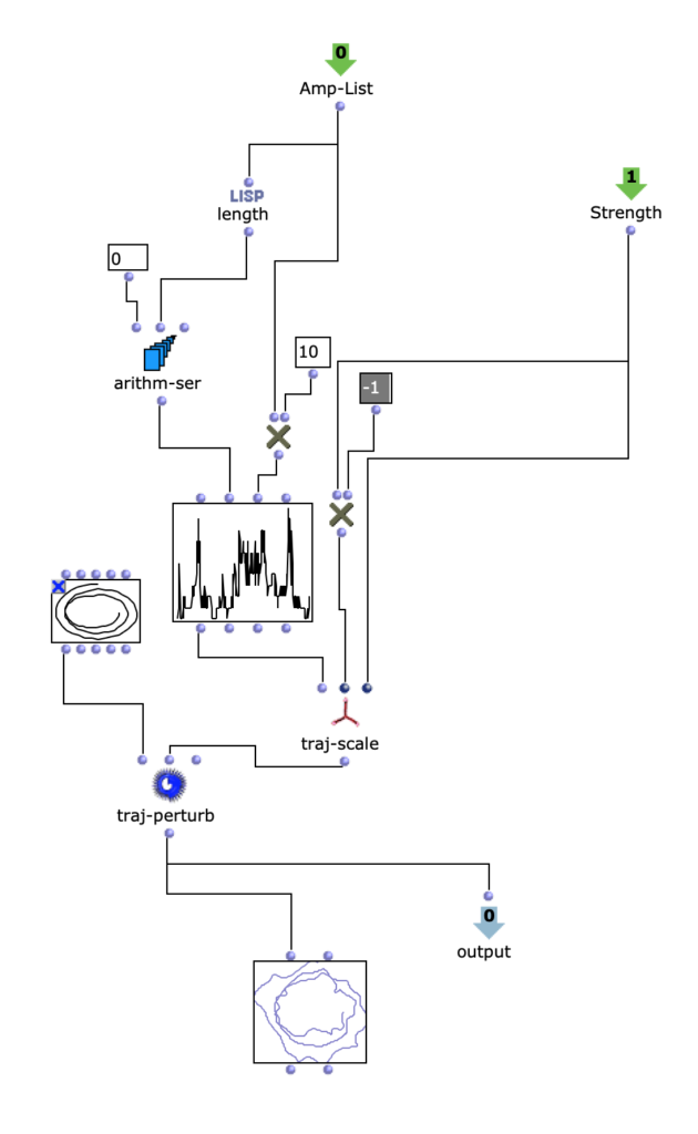
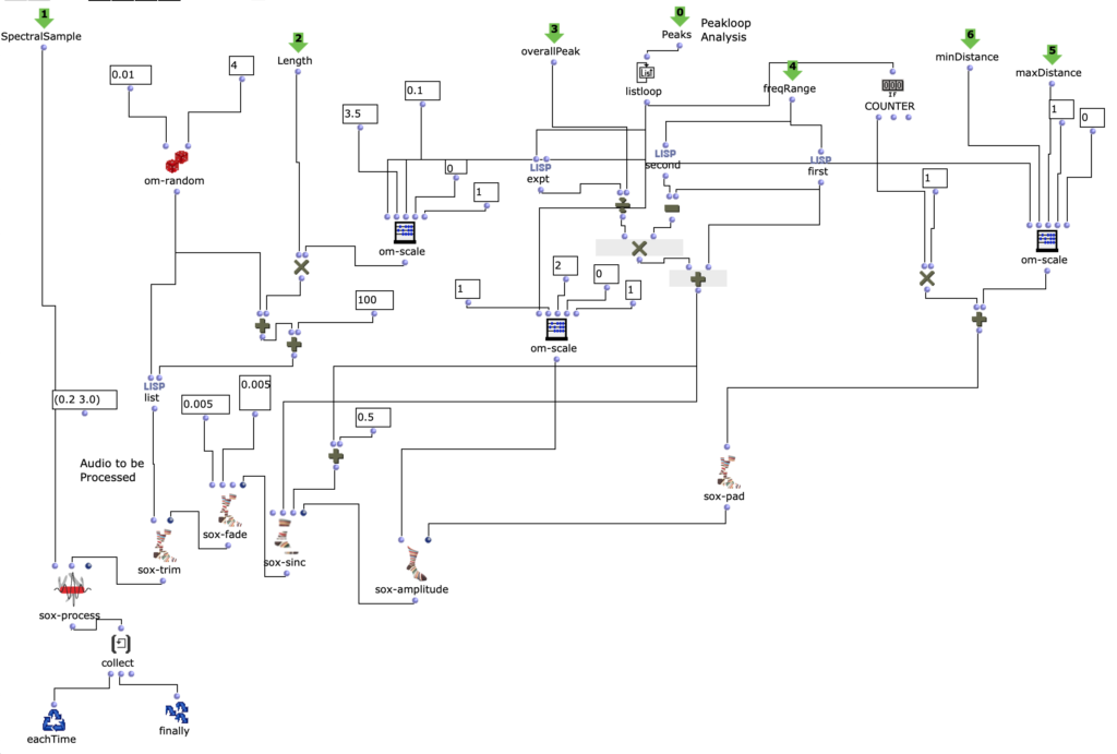
I present in this article residual – i, a three-minute solo piece for prepared piano commissioned as a companion work to John Cage’s Sonatas and Interludes for prepared piano. In analyzing Cage’s work and subsequently composing a companion to it, I employed a self-designed texture synthesis tool driven by machine learning clustering. The technical overview of that tool can be read at this other blogpost, or in the proceedings of the 2022 International Conference on Technologies for Music Notation and Representation (TENOR 2022). The blogpost you are reading now will briefly explain how that tool (and generally, music informatics) was applied in composing this short piano piece.
Background
John Cage’s Sonatas and Interludes (1946-48) is a 60-minute work for solo prepared piano that involves placing various objects (metal screws, bolts, nuts, pieces of plastic, rubber and eraser) in the strings of the piano. These objects ‚prepare‘ the piano, altering its sound and bringing out a variety of different, heterogenous timbres. Some keys produce chords, others buzz, or even have the pitch completely removed. The sound profile of the Sonatas and Interludes are arguably the work’s most iconic aspect.
However, the form of the Sonatas and Interludes is also noteworthy. The work consists of sixteen sonatas and four interludes, with most movements lasting somewhere between 1 and 4 minutes each. As part of an ongoing commissioning project, pianist and composer Amy Williams premieres new ‚interludes‘ which are placed amidst the existing sonatas and interludes by Cage. In early 2022 I received the opportunity to compose a short piece that would use a piano with Cage’s „preparations“, and would be inserted as an interlude amidst the sonatas and interludes of Cage’s work.
Approach
I was interested in composing a piece that acknowledged both the sound- and time-identity of the Sonatas and Interludes. While arguably the most iconic aspect of Cage’s Sonatas and Interludes is its sounds, I feel that the work’s form, it’s time-based content, is equally impactful. Many of the its movements are cast in AABB form, reflecting classical period sonatas. Additionally, the distribution of the individual sonatas and interludes take a symmetrical form: four groups of four sonatas each, partitioned by the four interludes:
Sonatas I–IV Interlude 1 Sonatas V–VIII Interludes 2–3 Sonatas IX–XII Interlude 4 Sonatas XIII–XVI
As a pre-compositional constraint, I decided that all sonorities in my piece would be taken/excerpted directly from the score of the Cage. To use the metaphor of a painter, the score of the Cage was my palette of colors, and not the prepared piano itself. This meant that not only every chord or single note in my piece would be excerpted from the Cage, it also meant that the chord or note’s particular duration would also be used in my piece. The sound and duration were joined as a single item. In a way, my piece was a form of granular synthesis, taking single-attack grains of the Sonatas and Interludes, and recontextualizing them in a new order.
Preprocessing
In order to observe and meaningfully comprehend all the individual sonorities in the 60-minute-long Cage, I used a simple machine learning clustering method to categorize all ~7k sonorities into 12 groups. Using my texture synthesis tool, I was not only able to organize audio features of these ~7k sonorities in a a visual editor, I was also able to export and listen to each individual sonority as a single, short audio file.
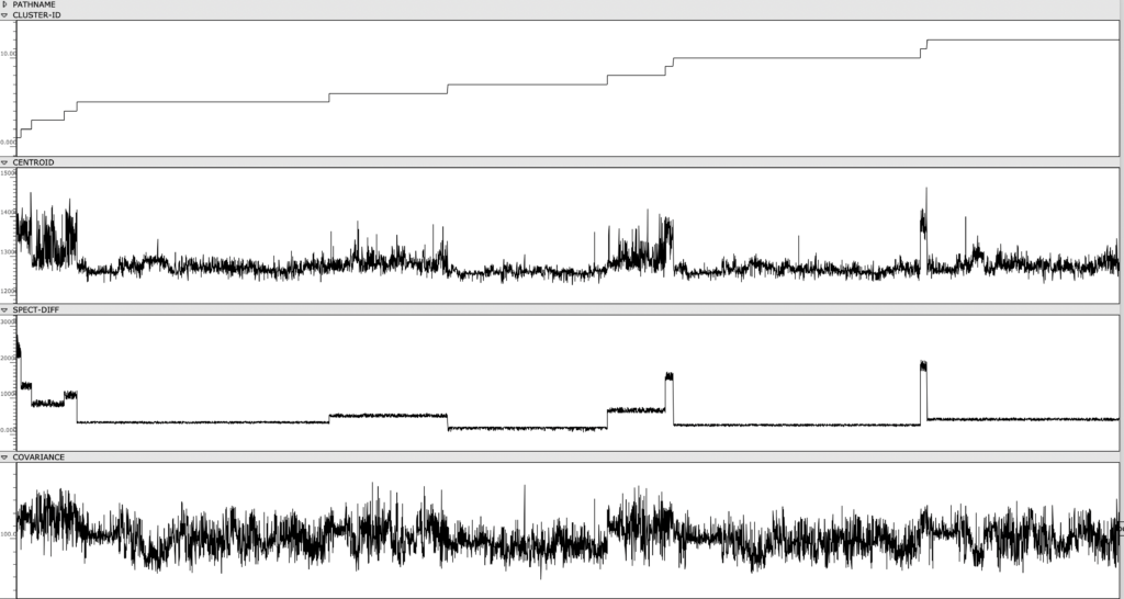
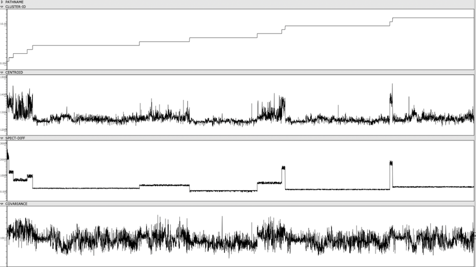
Figure 1: Clusters and audio features are visually represented and sorted, providing an out-of-time view of the Cage’s spectral content.
Once the sonorities have been extracted as individual transients, I used a k-means clustering method to sort these sonorities into 12 clusters. To briefly explain this machine learning method, the clustering algorithm receives a vector of several audio features as an input representing a sonority from the Cage (the audio features used were spectral centroid, spectral difference, and spectral covariance*). The algorithm then sorts these audio vectors into 12 groups, placing sounds with similar vector-values in the same group. This process in unsupervised, meaning it is not seeking to emulate a trained result that I predetermined. Rather, because these three audio features, as a trio, don’t represent any particularly given parameter in music, the algorithm returns clusters of sound that are correlated along multifaceted sound profiles that are aurally cohesive but not as simple as being sorted by a single parameter like pitch, duration, brightness, or noisiness.
Composition
My piece residual – i uses sonorities exclusively from clusters 2, 4, 9, 11. Referring back to the class-array figure, there is a clear line of differentiation between these clusters and the rest, correlated specifically to the spectral difference of the sonorities. These sonorities had an unusually high spectral difference, due either to their bright harmonic content (which creates a sharp delta between the attack and sustain of the transient) or their short duration (which creates a sharp delta between the attack and sustain/resonance of the transient). By placing each of these clusters in sequence, and the sounds within each cluster in sequence, this quality of shortness and brightness is clearly audible (see audio).
I treated this sequence as a kind of DNA for the piece. Large portions of it were copied into the score (sequences of around 20-30 transients. This process was done by hand, listening to each individual transient in the sequence, and looking up in the score of the Cage what the corresponding notes were). It was at this point that the machine learning methods involved in the piece are finished. From here, I began to sculpt and shape these longer sequences into shorter bursts. I also added repeat brackets at different moments, creating moments of ‚freeze‘ in the piece’s hurtling forward momentum.
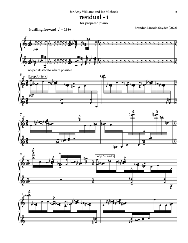
Figure 3a: Loop A designates the first several (circa 20) sonorities in the cluster sequence, looped over and over. This sequence served as a scaffolding from which the piece was composed around.
Figure 3b: This is the same page of the score, after notes have been removed, transforming the work into short bursts of sound.
Conclusion
Many of the cutting edge applications of machine learning in audio are towards the improvement of automated transcription, neural audio synthesis, and other tasks which have a clear goal and benchmark to test against. My particular application of machine learning in this piece is not for optimizing any task like this. Rather, the act of clustering audio served more as a means to explore the Sonatas and Interludes from a vantage point that I had not yet seen them from. Similar to my previous works that involve machine learning, being aware of how the machine learning methods are implemented is an essential first step in mindfully composing a work using such methods. As suggested by the title, residual – i serves as a proof of concept for a possible larger set of companion pieces, in which machine learning methods are used as a means to critically reexamine and „re-hear“ a familiar piece of music.
Listen to a full performance of residual – i here.
*These three features are measurements typically used to categorize the timbre and spectral content of an audio signal. The spectral centroid represents the center of mass in a spectrum. The spectral difference represents the average delta in energy between adjacent windows of the spectrum. The spectral covariance represents the spectral variability of a signal, i.e. how much the signal varies between its frequency bins.