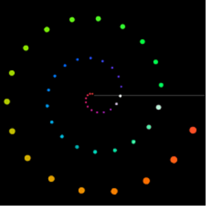
Die Whitney Music Box ist eine sonifizierte und/oder visuelle Darstellung einer Reihe zusammenhängender Sound-Elemente. Diese Elemente können musikalisch gesehen beispielsweise chromatisch oder harmonisch zusammenhängen. In der visuellen Darstellung wird jedes dieser Elemente mit einem Kreis oder Punkt dargestellt (siehe Abbildung 1). Diese Punkte kreisen je nach eigener zugewiesener Frequenz um einen gemeinsamen Mittelpunkt. Je kleiner die Frequenz, desto kleiner der Radius des Umlaufkreises und desto höher die Umlaufgeschwindigkeit. Jedes Sound-Element repräsentiert in einer harmonischen Reihe Vielfache einer festgelegten Grundfrequenz. Sobald ein Element einen Umlauf um den Mittelpunkt vollbracht hat wird der Sound mit der zu repräsentierenden Frequenz ausgelöst. Durch die mathematische Beziehung zwischen den einzelnen Elementen gibt es Momente während der Ausführung der Whitney Music Box in denen bestimmte Elemente gleichzeitig ausgelöst werden und Phasen, in denen die Elemente konsekutiv wahrgenommen werden können. Zu Anfang und am Ende werden alle Elemente gleichzeitig ausgelöst.
Abbildung 1: Whitney Music Box – visuelle Darstellung
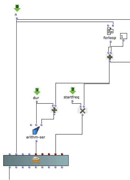
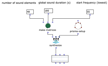
Im Rahmen dieses Projekts wird OMChroma für die Synthese der einzelnen Soundelemente verwendet (siehe Abbildung 2). Die Synthese-Klassen von OMChroma erben von OpenMusic’s class-array Objekt. Die Spalten in dem Array beschreiben die einzelnen Komponenten innerhalb der Synthese. Die Reihen repräsentieren Parameter, die den einzelnen Komponenten lokal oder dem gesamten Prozess global zugewiesen können. Für die Whitney Music Box werden Elemente gebraucht, die die einzelnen Tonhöhenabstufungen und die zeitliche Versetzung der einzelnen Tonhöhenabstufungen umsetzt. Dabei wird eine OMChroma-Matrix als Event angesehen. Ein solches Event repräsentiert eine Tonhöhe und die Sound-Wiederholungen innerhalb der globalen Dauer der Whitney Music Box. Die globale Dauer wird zu Anfang festgelegt und beschreibt zugleich die Umlaufzeit der niedrigsten Frequenz bzw. der zuvor festgelegten Startfrequenz. Jede Matrix repräsentiert eine Frequenz, die ein Vielfaches der Startfrequenz ist. Die Umlaufzeit eines Soundelements ergibt sich durch die Formel:
duration(global) / n
Dabei ist n der Index der einzelnen Soundelemente bzw. Matrizen. Je höher der Index, desto höher ist auch die Frequenz und desto kleiner die Umlaufzeit. Die Wiederholungen der Sound-Elemente, wird durch den Parameter e-dels festgelegt. Jede Komponente einer Matrix erhält ein unterschiedliches Entry-Delay. Diese Entry-Delays stehen in einem regelmäßigen Abstand von duration(global) / n zueinander.
Abbildung 2: Anwendung von OMChroma
Ohne Spatialisierung hört sich die Whitney Music Box mit OMChroma wie folgt an:
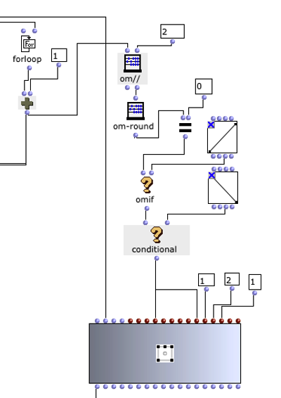
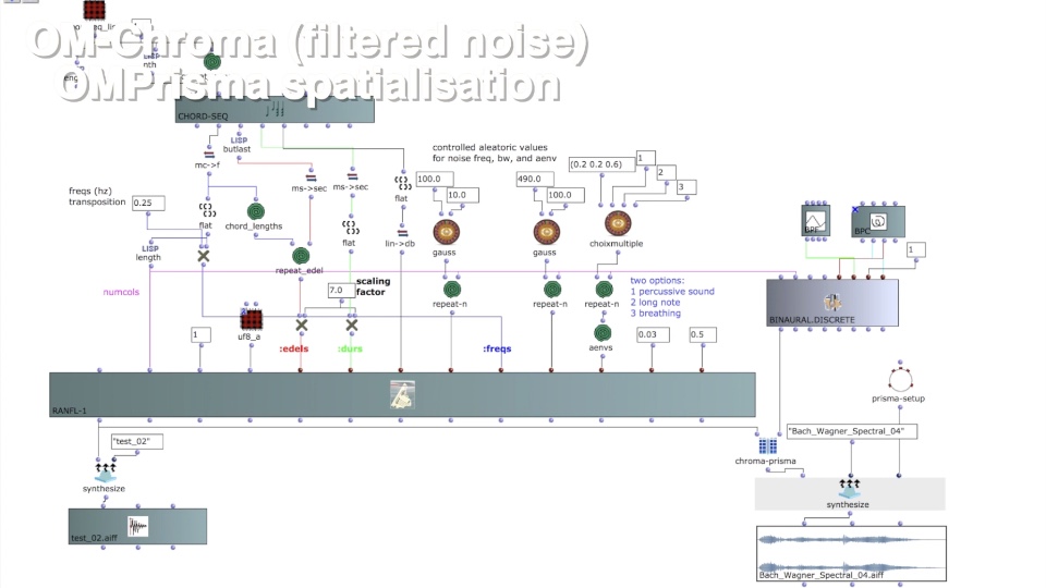
In Abbildung 3 wird dargestellt, wie die gesammelten Matrizen oder Sound-Events mit der Bibliothek OMPrisma spatialisiert werden. Dabei wurde sich an der visuellen Darstellung der Whitney Music Box orientiert. Dabei sind Sound-Elemente mit niedriger Frequenz weiter vom Mittelpunkt entfernt und Soundelemente mit hoher Frequenz kreisen umso näher um den Mittelpunkt. Mit OMPrisma soll diese Darstellung im Raumklang umgesetzt werden. Das heißt, Sounds mit niedriger Frequenz sollen sich weiter entfernt anhören und Sounds mit hoher Frequenz nah am Hörer. Im OpenMusic-Patch wurden zusätzlich Elemente mit geradem Index weiter nach vorne & weiter nach rechts positioniert und analog Elemente mit ungeradem Index weiter nach links und nach hinten positioniert, um die Sounds gleichmäßig im Raum zu verteilen. Die Klassen von OMPrisma bieten zudem noch Presets für die attenuation-function, air-absorption-function und time-of-flight-function an. Diese wurden eingesetzt, um zusätzlich zu der Positionierung im Raum noch mehr Gefühl von Räumlichkeit zu schaffen.
Abbildung 3: Anwendung von OMPrisma
In Stereo hört sich die Whitney Music Box beispielsweise wie folgt an:
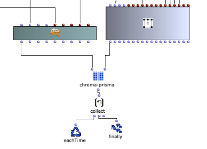
In Abbildung 4 wird dargestellt, wie die gesammelten OMChroma- und OMPrisma-Matrizen über die chroma-prisma-Funktion zusammengelegt. Die Liste aller gesammelten Matrizen werden über einen om-loop zurückgegeben und über die synthesize-Funktion als Sound gerendert (siehe Abbildung 5).
Abbildung 4: chroma-prisma
Abbildung 5: loop und synthesize
Der OpenMusic-Patch sowie Soundbeispiele können unter folgenden Links abgerufen werden:
Vorstellung des Projekts eines Alumni beim Ircam Forum 23 in Paris mit Software von Marlon Schumacher
Projektverantwortliche: Marco Bidin, Fernando Maglia
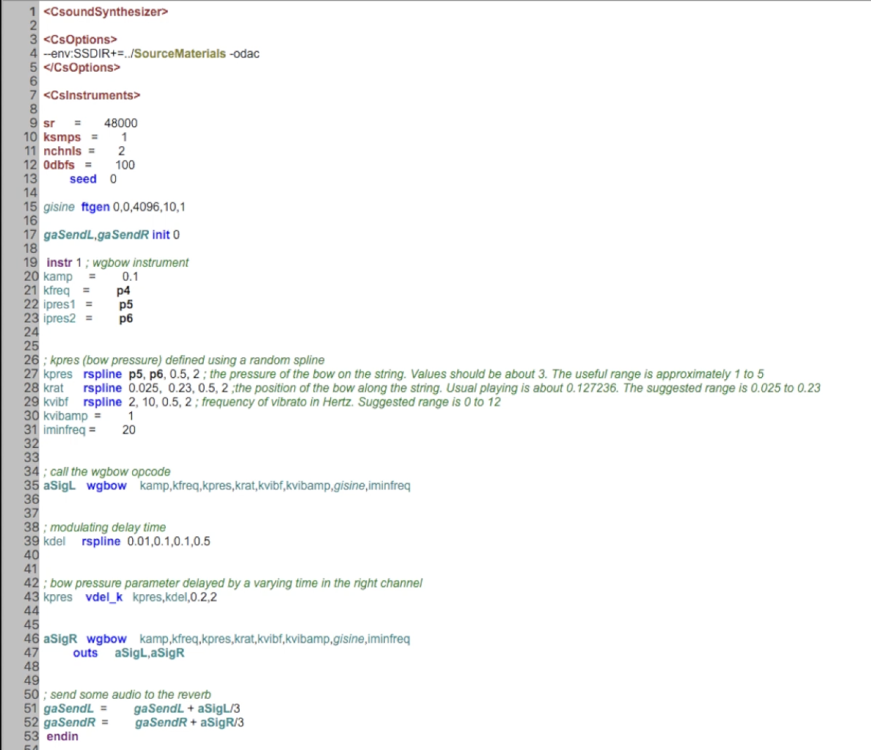
Im IRCAM-Forum im März 2023 in Paris (special edition zum Thema AR/VR Spatialization) hat der ehemalige Student und Mitarbeiter Marco Bidin Projekte zum Thema binaurale Klangsynthese vorgestellt, welche durch von Prof. Marlon Schumacher entwickelte Software realisiert wurden. Als Synthese-Werkzeuge kamen unter Anderem CSound, Cycling 74’s Max, OpenMusic mit der Library OMPrisma zum Einsatz, gemastert wurde in der DAW Logic Pro X. Die Klangsynthese verwendet teils subtraktive Ansätze, Waveguides und andere physikalische Modelle.
Ausschnitt eines in Csound implementierten Orchesters.
Music for Headphones III ist eine Produktion von ALEA, Associazione Laboratorio Espressioni Artistiche.
SKAS-Symbolische Klangverarbeitung und Analyse/Synthese
Prof. Dr. Marlon Schumacher
Zwischenprojekt von Andres Kaufmes
HfM Karlsruhe – IMWI (Institut für Musikinformatik und Musikwissenschaft)
WiSe 2022/23
_____________
Für dieses Zwischenprojekt habe ich mich mit der Implementierung eines Transient- Prozessors in OpenMusic mit Hilfe der OM-Sox Library beschäftigt.
Mit einem Transient Prozessor (auch Transient Designer oder Transient Shaper) lässt sich das Ein- und Ausschwingverhalten (Attack/Release) der Transienten eines Audiosignal beeinflussen.
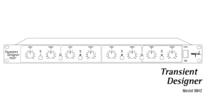
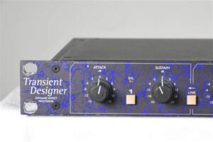
Das erste vorgestellte Hardware Gerät war der 1998 von der Firma SPL vorgestellte SPL TD4, welcher als 19″ Rack-Gerät erhältlich war und in fortgeschrittener Version bis heute erhältlich ist.
Transient Designer der Firma SPL. (c) SPL
Transient Designer eignen sich besonders für die Bearbeitung von perkussiven Klängen oder auch für Sprache. Zunächst müssen die Transienten aus dem gewünschten Audiosignal isoliert werden, dies lässt sich zum Beispiel mit Hilfe eines Kompressors umsetzen. Durch eine kurze Attack-Zeit werden die Transienten „geduckt“ und das Signal kann vom Original abgezogen werden. Anschließend kann das Audiosignal im Verlauf der Signalkette mit weiteren Effekten bearbeitet werden.
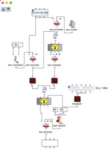
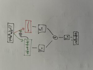
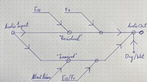
Transient-Prozessor Patch. FX- Kette der beiden Signalwege (links „Transient“, rechts „Residual“).
Im Patch zu sehen ist an oberster Stelle die zu bearbeitende Audiodatei, von welcher, wie eben beschrieben, mit Hilfe eines Kompressors die Transienten isoliert, und das resultierende Signal vom originalen abgezogen wird. Nun werden zwei Signalwege gebildet: Die isolierten Transienten werden in der linken „Kette“ verarbeitet, das residuale Signal in der rechten. Nachdem beide Signalwege mit Audioeffekten bearbeitet wurden, werden sie zusammengemischt, wobei das Mischverhältnis (Dry/Wet) beider Signalwege nach belieben eingestellt werden kann. Am Ende der Signalverarbeitung befinden sich ein globaler Reverb-Effekt.
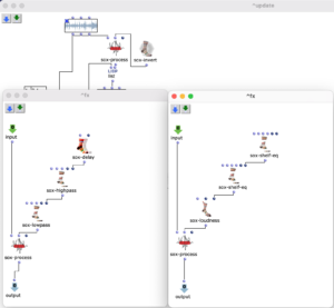
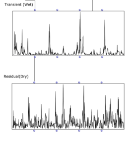
„Scope“ Ansicht der beiden Signalwege. Skizzen zum möglichen Signalweg und Verarbeitung.
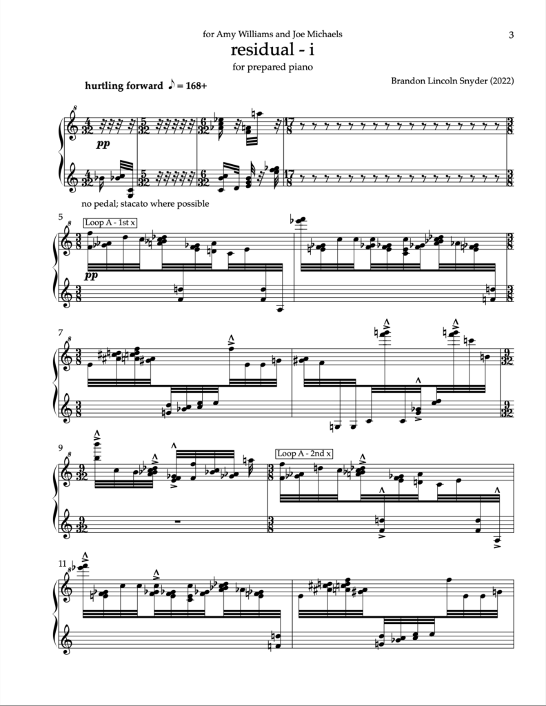
I present in this article residual – i, a three-minute solo piece for prepared piano commissioned as a companion work to John Cage’s Sonatas and Interludes for prepared piano. In analyzing Cage’s work and subsequently composing a companion to it, I employed a self-designed texture synthesis tool driven by machine learning clustering. The technical overview of that tool can be read at this other blogpost, or in the proceedings of the 2022 International Conference on Technologies for Music Notation and Representation (TENOR 2022). The blogpost you are reading now will briefly explain how that tool (and generally, music informatics) was applied in composing this short piano piece.
Background
John Cage’s Sonatas and Interludes (1946-48) is a 60-minute work for solo prepared piano that involves placing various objects (metal screws, bolts, nuts, pieces of plastic, rubber and eraser) in the strings of the piano. These objects ‚prepare‘ the piano, altering its sound and bringing out a variety of different, heterogenous timbres. Some keys produce chords, others buzz, or even have the pitch completely removed. The sound profile of the Sonatas and Interludes are arguably the work’s most iconic aspect.
However, the form of the Sonatas and Interludes is also noteworthy. The work consists of sixteen sonatas and four interludes, with most movements lasting somewhere between 1 and 4 minutes each. As part of an ongoing commissioning project, pianist and composer Amy Williams premieres new ‚interludes‘ which are placed amidst the existing sonatas and interludes by Cage. In early 2022 I received the opportunity to compose a short piece that would use a piano with Cage’s „preparations“, and would be inserted as an interlude amidst the sonatas and interludes of Cage’s work.
Approach
I was interested in composing a piece that acknowledged both the sound- and time-identity of the Sonatas and Interludes. While arguably the most iconic aspect of Cage’s Sonatas and Interludes is its sounds, I feel that the work’s form, it’s time-based content, is equally impactful. Many of the its movements are cast in AABB form, reflecting classical period sonatas. Additionally, the distribution of the individual sonatas and interludes take a symmetrical form: four groups of four sonatas each, partitioned by the four interludes:
As a pre-compositional constraint, I decided that all sonorities in my piece would be taken/excerpted directly from the score of the Cage. To use the metaphor of a painter, the score of the Cage was my palette of colors, and not the prepared piano itself. This meant that not only every chord or single note in my piece would be excerpted from the Cage, it also meant that the chord or note’s particular duration would also be used in my piece. The sound and duration were joined as a single item. In a way, my piece was a form of granular synthesis, taking single-attack grains of the Sonatas and Interludes, and recontextualizing them in a new order.
Preprocessing
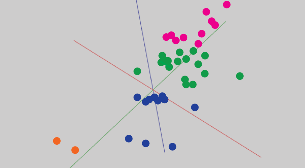
In order to observe and meaningfully comprehend all the individual sonorities in the 60-minute-long Cage, I used a simple machine learning clustering method to categorize all ~7k sonorities into 12 groups. Using my texture synthesis tool, I was not only able to organize audio features of these ~7k sonorities in a a visual editor, I was also able to export and listen to each individual sonority as a single, short audio file.
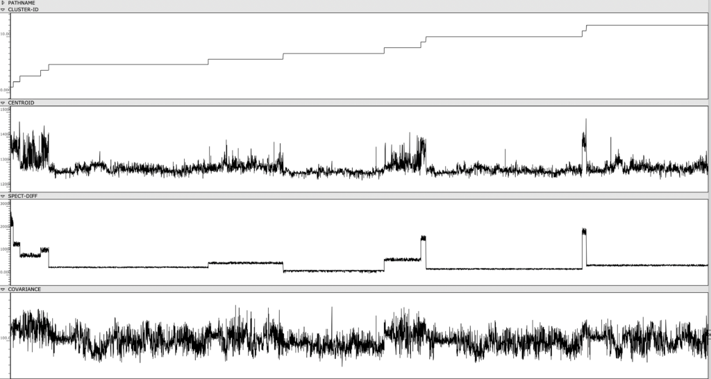
Figure 1: Clusters and audio features are visually represented and sorted, providing an out-of-time view of the Cage’s spectral content.
Once the sonorities have been extracted as individual transients, I used a k-means clustering method to sort these sonorities into 12 clusters. To briefly explain this machine learning method, the clustering algorithm receives a vector of several audio features as an input representing a sonority from the Cage (the audio features used were spectral centroid, spectral difference, and spectral covariance*). The algorithm then sorts these audio vectors into 12 groups, placing sounds with similar vector-values in the same group. This process in unsupervised, meaning it is not seeking to emulate a trained result that I predetermined. Rather, because these three audio features, as a trio, don’t represent any particularly given parameter in music, the algorithm returns clusters of sound that are correlated along multifaceted sound profiles that are aurally cohesive but not as simple as being sorted by a single parameter like pitch, duration, brightness, or noisiness.
Composition
My piece residual – i uses sonorities exclusively from clusters 2, 4, 9, 11. Referring back to the class-array figure, there is a clear line of differentiation between these clusters and the rest, correlated specifically to the spectral difference of the sonorities. These sonorities had an unusually high spectral difference, due either to their bright harmonic content (which creates a sharp delta between the attack and sustain of the transient) or their short duration (which creates a sharp delta between the attack and sustain/resonance of the transient). By placing each of these clusters in sequence, and the sounds within each cluster in sequence, this quality of shortness and brightness is clearly audible (see audio).
I treated this sequence as a kind of DNA for the piece. Large portions of it were copied into the score (sequences of around 20-30 transients. This process was done by hand, listening to each individual transient in the sequence, and looking up in the score of the Cage what the corresponding notes were). It was at this point that the machine learning methods involved in the piece are finished. From here, I began to sculpt and shape these longer sequences into shorter bursts. I also added repeat brackets at different moments, creating moments of ‚freeze‘ in the piece’s hurtling forward momentum.
Figure 3a: Loop A designates the first several (circa 20) sonorities in the cluster sequence, looped over and over. This sequence served as a scaffolding from which the piece was composed around.
Figure 3b: This is the same page of the score, after notes have been removed, transforming the work into short bursts of sound.
Conclusion
Many of the cutting edge applications of machine learning in audio are towards the improvement of automated transcription, neural audio synthesis, and other tasks which have a clear goal and benchmark to test against. My particular application of machine learning in this piece is not for optimizing any task like this. Rather, the act of clustering audio served more as a means to explore the Sonatas and Interludes from a vantage point that I had not yet seen them from. Similar to my previous works that involve machine learning, being aware of how the machine learning methods are implemented is an essential first step in mindfully composing a work using such methods. As suggested by the title, residual – i serves as a proof of concept for a possible larger set of companion pieces, in which machine learning methods are used as a means to critically reexamine and „re-hear“ a familiar piece of music.
Listen to a full performance of residual – i here.
*These three features are measurements typically used to categorize the timbre and spectral content of an audio signal. The spectral centroid represents the center of mass in a spectrum. The spectral difference represents the average delta in energy between adjacent windows of the spectrum. The spectral covariance represents the spectral variability of a signal, i.e. how much the signal varies between its frequency bins.
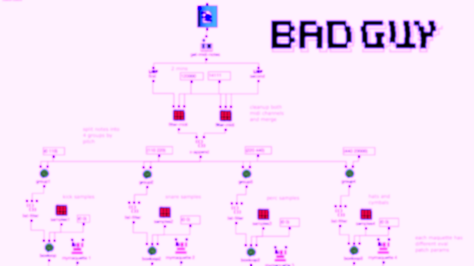
Inspiriert vom „Infinite Bad Guy“ Projekt und all den sehr unterschiedlichen Versionen, wie manche Leute ihre Fantasie zu diesem Song beflügelt haben, dachte ich, vielleicht könnte ich auch damit experimentieren, eine sehr lockere, instrumentale Coverversion von Billie Eilish’s „Bad Guy“ zu erstellen.
Betreuer: Prof. Dr. Marlon Schumacher
Eine Studie von: Kaspars Jaudzems
Wintersemester 2021/22
Hochschule für Musik, Karlsruhe
Zur Studie:
Ursprünglich wollte ich mit 2 Audiodateien arbeiten, eine FFT-Analyse am Original durchführen und dessen Klanginhalt durch Inhalt aus der zweiten Datei „ersetzen“, lediglich basierend auf der Grundfrequenz. Nachdem ich jedoch einige Tests mit einigen Dateien durchgeführt hatte, kam ich zu dem Schluss, dass diese Art von Technik nicht so präzise ist, wie ich es gerne hätte. Daher habe ich mich entschieden, stattdessen eine MIDI-Datei als Ausgangspunkt zu verwenden.
Sowohl die erste als auch die zweite Version meines Stücks verwendeten nur 4 Samples. Die MIDI-Datei hat 2 Kanäle, daher wurden 2 Dateien zufällig für jede Note jedes Kanals ausgewählt. Das Sample wurde dann nach oben oder unten beschleunigt, um dem richtigen Tonhöhenintervall zu entsprechen, und zeitlich gestreckt, um es an die Notenlänge anzupassen.
Die zweite Version meines Stücks fügte zusätzlich einige Stereoeffekte hinzu, indem 20 zufällige Pannings für jede Datei vor-generiert wurden. Mit zufällig angewendeten Kammfiltern und Amplitudenvariationen wurde etwas mehr Nachhall und menschliches Gefühl erzeugt.
Akusmatische Studie Version 1
Akusmatische Studie Version 2
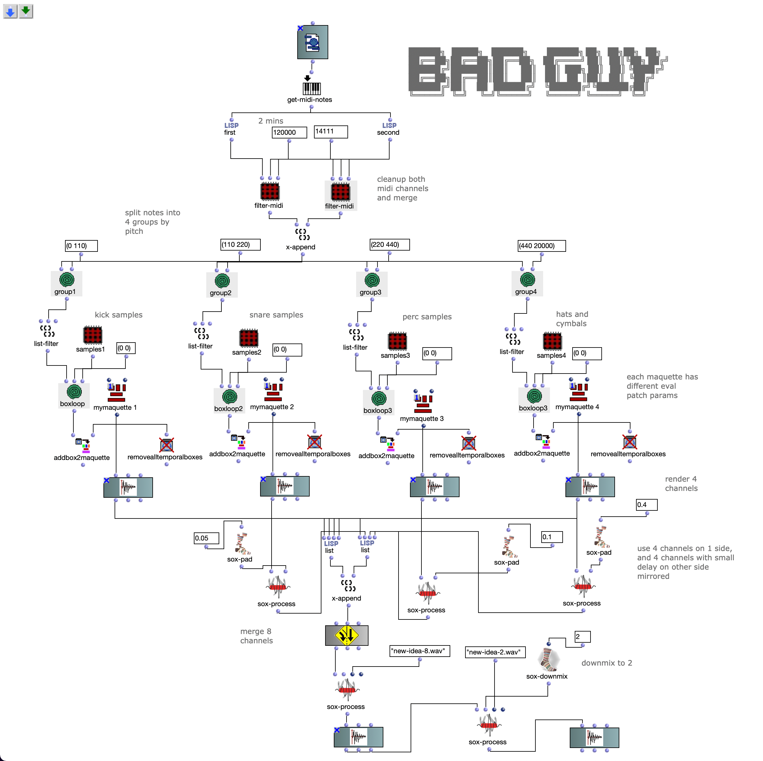
Die dritte Version war eine viel größere Änderung. Hier werden die Noten beider Kanäle zunächst nach Tonhöhe in 4 Gruppen eingeteilt. Jede Gruppe umfasst ungefähr eine Oktave in der MIDI-Datei.
Dann wird die erste Gruppe (tiefste Töne) auf 5 verschiedene Kick-Samples abgebildet, die zweite auf 6 Snares, die dritte auf perkussive Sounds wie Agogo, Conga, Clap und Cowbell und die vierte Gruppe auf Becken und Hats, wobei insgesamt etwa 20 Samples verwendet werden. Hier wird eine ähnliche Filter-und-Effektkette zur Stereoverbesserung verwendet, mit dem Unterschied, dass jeder Kanal fein abgestimmt ist. Die 4 resultierenden Audiodateien werden dann den 4 linken Audiokanälen zugeordnet, wobei die niedrigeren Frequenzen kanale zur Mitte und die höheren kanale zu den Seiten sortiert werden. Für die anderen 4 Kanäle werden dieselben Audiodateien verwendet, aber zusätzliche Verzögerungen werden angewendet, um Bewegung in das Mehrkanalerlebnis zu bringen.
Akusmatische Studie Version 3
Die 8-Kanal-Datei wurde auf 2 Kanäle in 2 Versionen heruntergemischt, einer mit der OM-SoX-Downmix-Funktion und der andere mit einem Binauralix-Setup mit 8 Lautsprechern.
Akusmatische Studie Version 3 – Binauralix render
Erweiterung der akousmatischen Studie – 3D 5th-order Ambisonics
Die Idee mit dieser Erweiterung war, ein kreatives 36-Kanal-Erlebnis desselben Stücks zu schaffen, also wurde als Ausgangspunkt Version 3 genommen, die nur 8 Kanäle hat.
Ausgangspunkt Version 3
Ich wollte etwas Einfaches machen, aber auch die 3D-Lautsprecherkonfiguration auf einer kreativen weise benutzen, um die Energie und Bewegung, die das Stück selbst bereits gewonnen hatte, noch mehr hervorzuheben. Natürlich kam mir die Idee in den Sinn, ein Signal als Quelle für die Modulation von 3D-Bewegung oder Energie zu verwenden. Aber ich hatte keine Ahnung wie…
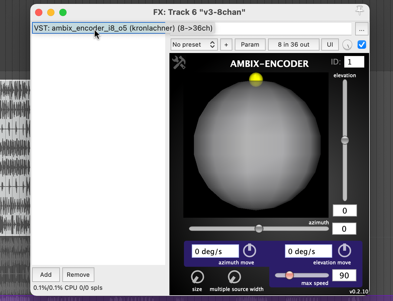
Plugin „ambix_encoder_i8_o5 (8 -> 36 chan)“
Bei der Recherche zur Ambix Ambisonic Plugin (VST) Suite bin ich auf das Plugin „ambix_encoder_i8_o5 (8 -> 36 chan)“ gestoßen. Dies schien aufgrund der übereinstimmenden Anzahl von Eingangs- und Ausgangskanälen perfekt zu passen. In Ambisonics wird Raum/Bewegung aus 2 Parametern übersetzt: Azimuth und Elevation. Energie hingegen kann in viele Parameter übersetzt werden, aber ich habe festgestellt, dass sie am besten mit dem Parameter Source Width ausgedrückt wird, weil er die 3D-Lautsprecherkonfiguration nutzt, um tatsächlich „nur“ die Energie zu erhöhen oder zu verringern.
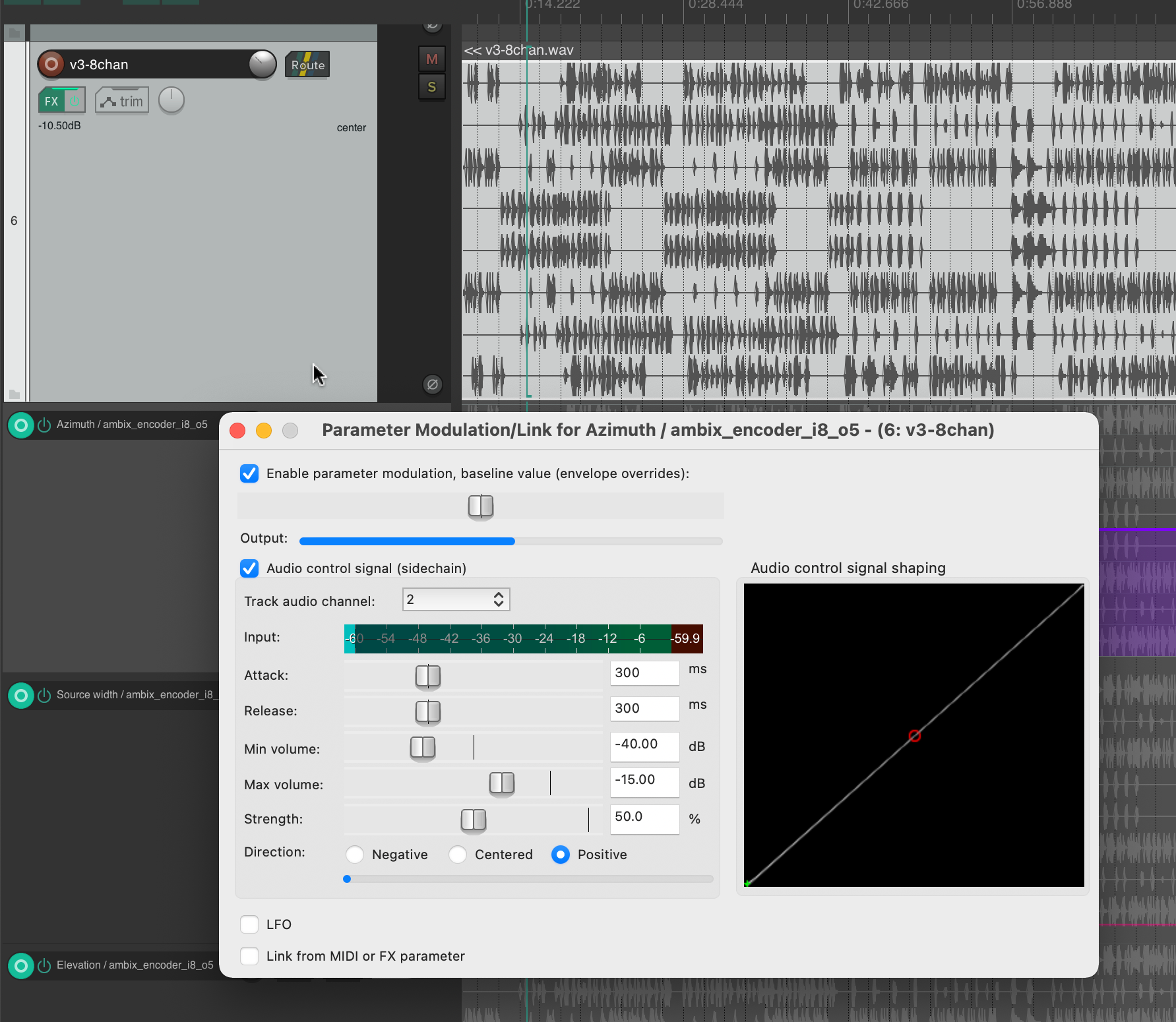
Da ich wusste, welche Parameter ich modulieren muss, begann ich damit zu experimentieren, verschiedene Spuren als Quelle zu verwenden. Ehrlich gesagt war ich sehr froh, dass das Plugin nicht nur sehr interessante Klangergebnisse lieferte, sondern auch visuelles Feedback in Echtzeit. Bei der Verwendung beider habe ich mich darauf konzentriert, ein gutes visuelles Feedback zu dem zu haben, was im Audiostück insgesamt vor sich geht.
Dies half mir, Kanal 2 für Azimuth, Kanal 3 für Source Width und Kanal 4 für Elevation auszuwählen. Wenn wir diese Kanäle auf die ursprüngliche Eingabe-Midi-Datei zurückverfolgen, können wir sehen, dass Kanal 2 Noten im Bereich von 110 bis 220 Hz, Kanal 3 Noten im Bereich von 220 bis 440 Hz und Kanal 4 Noten im Bereich von 440 bis 20000 Hz zugeordnet ist. Meiner Meinung nach hat diese Art der Trennung sehr gut funktioniert, auch weil die Sub-bass frequenzen (z. B. Kick) nicht moduliert wurden und auch nicht dafur gebraucht waren. Das bedeutete, dass der Hauptrhythmus des Stücks als separates Element bleiben konnte, ohne den Raum oder die Energiemodulationen zu beeinflussen, und ich denke, das hat das Stück irgendwie zusammengehalten.
Akusmatische Studie Version 4 – 36 channels, 3D 5th-order Ambisonics – Datei war zu groß zum Hochladen
Abstract: Spectral Select erkundet den spektralen Inhalt des einen, sowie den Amplitudenverlauf eines zweiten Samples und vereinigt diese in einem neuen musikalischen Kontext. Der durch Iteration entstehende meditative Charakter des Outputs wird durch lautere Amplituden-Peaks sowohl kontrastiert, als auch strukturiert. In einer überarbeiteten Version wurde Spectral Select im Ambisonics HOA-5 Format spatialisiert.
Betreuer: Prof. Dr. Marlon Schumacher
Eine Studie von: Anselm Weber
Wintersemester 2021/22 Hochschule für Musik, Karlsruhe
Zur Studie: In welchen Ausdrucksformen äußert sich die Verbindung zwischen Frequenz und Amplitude ? Sind beide Bereiche intrinsisch miteinander Verbunden und wenn ja, was könnten Ansätze sein, diese Ordnung neu zu gestalten ? Derartige Fragen beschäftigen mich bereits seid einiger Zeit. Daher ist der Versuch ebendieser Neugestaltung Kernthema bei Spectral Select. Inspiriert wurde ich dazu von AudioSculpt von IRCAM, welches wir in unserem Kurs: „Symbolische Klangverarbeitung und Analyse/Synthese“ gemeinsam mit Prof. Dr. Marlon Schumacher und Brandon L. Snyder kennenlernten und zum Teil nachbauten.
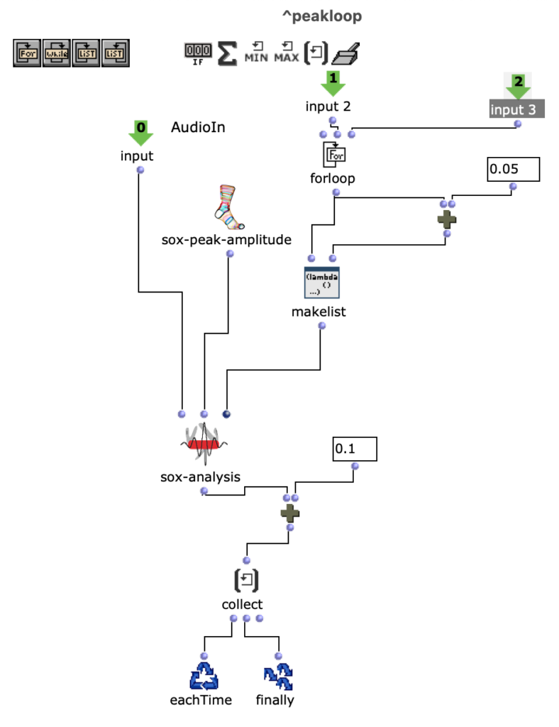
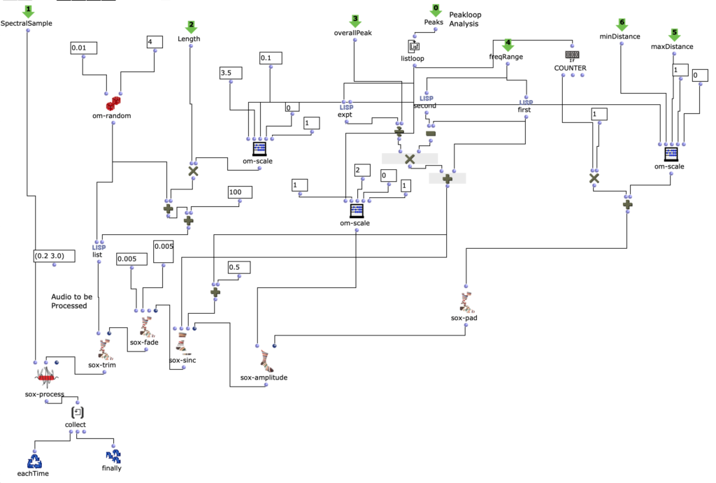
Spectral Edit funktioniert nach einem ähnlichen Prinzip, doch anstatt interessante Bereiche innerhalb eines Spektrums eines Samples von einem Benutzer herausarbeiten zu lassen, wurde entschieden, ein zweites Audiosample heranzuziehen. Dieses weitere Sample (im Verlauf dieses Artikels ab sofort als „Amplitudenklang“) bestimmt durch seinen Verlauf, wie das erste Sample (ab sofort als „Spektralklang“) durch OM-Sox verarbeitet werden soll. Um dies zu erreichen wird mit zwei Loops gearbeitet: Zunächst werden im ersteren „peakloop“ einzelne Amplitudenpeaks aus dem Amplitudenklang herausanalysiert. Daraufhin dient diese Analyse im Herzstück des Patches, dem „choosefreq“ Loop zur Auswahl interessanter Teilbereiche aus dem Spektralsample. Lautstarke Peaks filtern hierbei schmalere Bänder aus höheren Frequenzbereichen und bilden einen Kontrast zu schwächeren Peaks, welche etwas breiter Bänder aus tieferen Frequenzbereichen filtern.
peakloop – Analyse
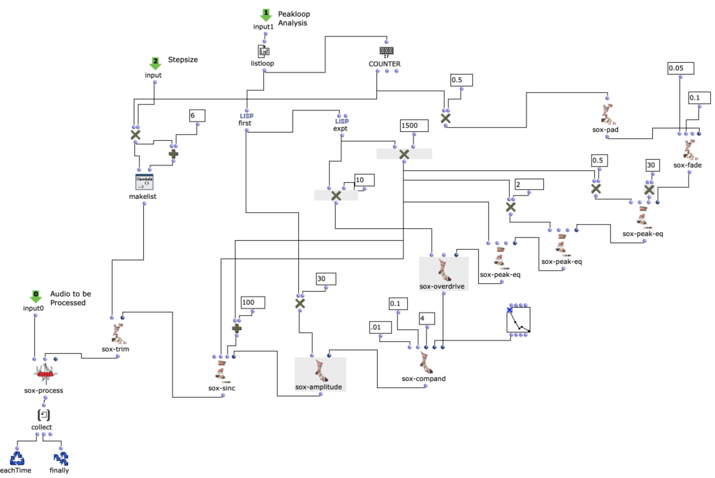
choosefreq Loop – Audio Processing
Wie klein die jeweiligen Iterationsschritte sind, wirkt sich dabei sowohl auf die Länge, als auch auf die Auflösung des gesamten Outputs aus. So können je nach Sample-Material sehr viele kurze Grains oder weniger, aber dafür längere Teilabschnitte erstellt werden. Beide dieser Parameter sind jedoch frei und unabhängig voneinander wählbar.
Im beigefügten Stück wurde sich beispielsweise für eine relativ hohe Auflösung (also eine erhöhte Anzahl an Iterationsschritten) in Kombination mit längerer Dauer des ausgeschnittenem Samples entschieden. Dadurch entsteht ein eher meditativer Charakter, wobei kein Teilabschnitt zu 100% dem anderen gleichen wird, da es ständig minimale Veränderungen unter den Peak-Amplituden des Amplitudenklangs gibt. Das noch relativ rohe Ergebnis dieses Algorithmus ist die erste Version meiner akusmatischen Studie.
Akusmatische Studie Version 1
Der darauffolgende Überarbeitungsschritt galt vor allem einer präziseren Herausarbeitung der Unterschiede zwischen den einzelnen Iterationsschritten. Dazu wurde eine Reihe an Effekten eingesetzt, welche sich wiederum je nach Peak-Amplitude des Amplitudenklangs unterschiedlich verhalten. Um dies zu ermöglichen, wurde die Effektreihe direkt in den Peakloop integriert.
Akusmatische Studie Version 2
Im dritten und letztem Überarbeitungsschritt erfolgte die Spatialisierung des Audios auf 8 Kanäle. Hierbei klingen die einzelnen Kanäle ineinander und ändern ihre Position im Uhrzeigersinn. Somit bleibt der Grundcharakter des Stückes bestehen, jedoch ist es nun zusätzlich möglich, das „Durcharbeiten“ des choosefreq Loops räumlich zu verfolgen. Damit diese Räumlichkeit erhalten bleibt, wurde der Output anschließend mithilfe von Binauralix für den Upload in binaural Stereo umgewandelt.
Akusmatische Studie Version 3 – Binaural
Spectral Select – Ambisonics
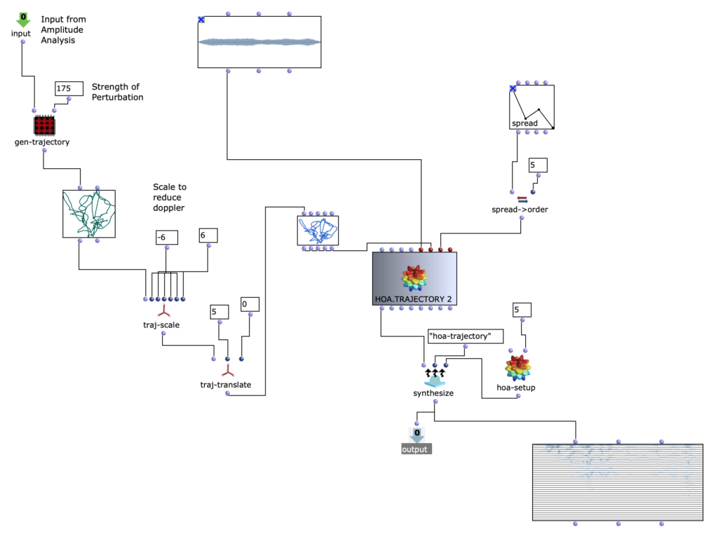
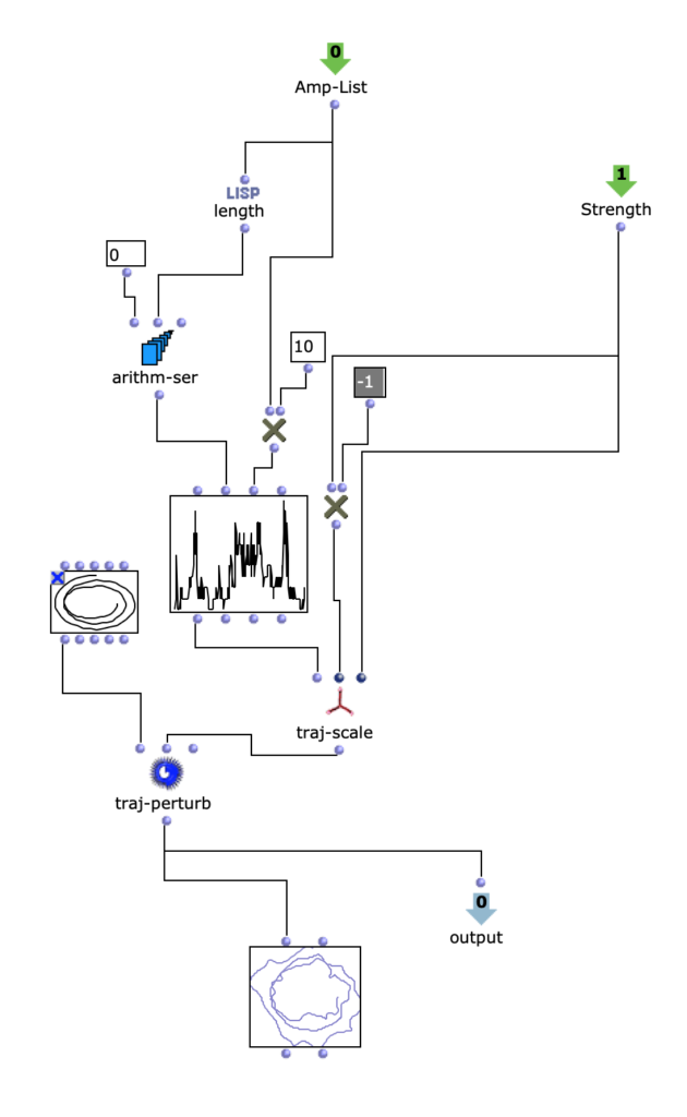
Im Zuge einer weiteren Überarbeitung wurde Spectral Select über die spatialisation class „Hoa-Trajectory“ von OM-Prisma neu spatialisiert und in das Ambisonics Format gebracht. Damit sich dieser Schritt konzeptionell und klanglich gut in die bisherigen Bearbeitungen eingliedert, soll der Amplitudenklang auch bei der Raumposition eine wichtige Rolle spielen. Die Möglichkeiten mithilfe von Open-Music und OM-Prisma Klänge zu spatialisieren sind zahlreich. Letzten Endes wurde entschieden, mit Hoa-Trajectory zu arbeiten. Hierbei ist die Klangquelle nicht an eine feste Position im Raum gebunden und kann mit einer Trajektorie beschrieben werden, welche auf die Gesamtdauer des Audio-Inputs skaliert wird.
Spatialisierung mit HOA.TRAEJECTORY
Die Trajektorie wird in Abhängigkeit der Amplituden-Analyse im vorhergehenden Schritt erstellt. Dabei wird eine simple, dreidimensionale Kreis Bewegung, welche sich in Spiralbewegung nach unten dreht, mit einer komplexeren, zweidimensionalen Kurve perturbiert. Die Y-Werte der komplexeren Kurve entsprechen dabei den herausanalysierten Amplitudenwerten des Amplitudenklanges. Somit ergeben sich je nach skalierung der Amplitudenkurve mehr oder weniger starke Abweichungen der Kreisbewegung. Höhere Amplitudenwerte sorgen also für ausuferndere Bewegungen im Raum.
Interessant hierbei ist, dass OM-Prisma auch Doppler-Effekte mitberücksichtigt. Dadurch ist zusätzlich hörbar, dass bei höheren Amplitudenwerten extremere Abstände zur Hörposition in der selben Zeit zurückgelegt werden. Dadurch nimmt dieser Arbeitsschritt unmittelbar Einfluss auf die Klangfarbe des gesamten Stückes. Je nach Skalierung der Trajektorie können schnelle Bewegungen dadurch stark überbetont werden, allerdings können (ab einer zu großen Entfernung) auch Artfakten entstehen. Damit ein besserer Eindruck Ensteht folgen 2 verschiedene durchläufe des Algorithmus mit unterschiedlichen Abständen zum Hörer.
Version mit extremen Doppler Effekten wodurch Artfakte enstehen können – Binaural Stereo
Version mit näherem Abstand und moderateren Doppler Effekten– Binaural Stereo
Spektralklang sowie Amplitudenklang wurden in diesem Beispiel im Gegensatz zu den vorherigen Klangbeispielen ausgetauscht. Es handelt sich hierbei um ein längeres Soundfile zur Analyse der Amplituden und einen weniger verzerrten Drone als Spektralklang. Die Idee hinter diesem Projekt ist ohnehin, mit verschiedenen Klangdateien zu experimentieren. Daher wurde auch der alter Algorithmus noch einmal überarbeitet um mehr Flexibilität bei unterschiedlichen Klangdateien zu bieten:
Überarbeitete skalierbare Version des alten Algorthimus zur Auswahl aus dem Spektralklang
Außerdem wird nun aus dem Spektralklang auf der Zeitachse randomisiert ausgewählt. Dadurch soll jeglicher formgebender Zusammenhang aus der Magnitude des Amplitudenklangs stammen und jegliche Klangfarbe aus dem Spektralklang extrahiert werden.
A link to download the applications can be found at the end of this blogpost. This project was also presented as a paper at the 2022 International Conference on Technologies for Music Notation and Representation (TENOR 2022).
Modularity in Sound Synthesis Tools
This blogpost walks through the structure and usage of two applications of machine learning (ML) methods for sound notation and synthesis. The first application is a modular sample replacement engine that uses a supervised classification algorithm to segment and transcribe a drum beat, and then reconstruct that same drum beat with different samples. The second application is a texture synthesis engine that uses an unsupervised clustering algorithm to analyze and sort large numbers of audio files.
The applications were developed in OpenMusic using the OM-SoX modular synthesis/analysis framework. This was so that the applications could be as modular as possible. Modular, meaning that they could be customized, extended, and integrated into a user’s own OpenMusic workflow. We believe this modularity offers something new to the community of ML and sound synthesis/analysis tools currently available. The approach to sound synthesis and analysis used here involves reading and querying many separate audio files. Such an approach can be encompassed by the larger term of „corpus-based concatenative synthesis/analysis,“ for which there are already several effective tools: the Caterpillar System, Audioguide, and OM-Pursuit. Additionally, OM-AI, ml.*, and zsa.descriptors are existing toolkits that integrate ML methods into Computer-Aided Composition (CAC) environments. While these tools are very precise, the internal workings of them are not immediately clear. By seeking for our applications to be modular, we mean that they can be edited, extended and integrated into existing CAC programs. It also means that they can be opened and up, examined, and reverse-engineered for a user’s own education.
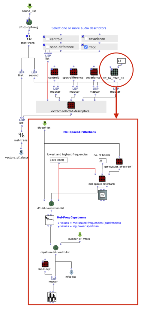
One example of this is in figure 1, our audio analysis engine. Audio descriptors are implemented as subpatches in lambda mode, and can be selected as needed for the input audio.
Figure 1: Interchangeable audio descriptors are set as patches in lambda mode. Here, a patch extracting 13 MFCCs is being used.
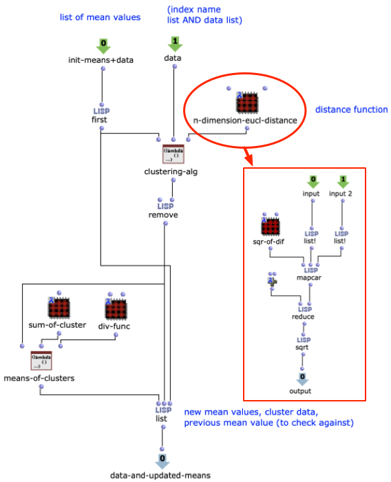
Another example is in figure 2, a customizable distance function in our texture synthesis application. This is the ML clustering algorithm that drives the application. Being a patch built from smaller OpenMusic objects, it is not only a tool for visualizing the algorithm at work, it also allows a user to edit it. For example, the n-dimension euclidean distance function could be substituted with another distance function, if needed.
Figure 2: A simple k-means clustering algorithm, built within an OpenMusic abstraction. The distance function takes the form of a subpatcher in lambda mode.
With the modularity of the project introduced, we will on the next page move on to the two specific applications.
Bis letzten August, waren meine Vorstellung zu Anwendungen maschinellen Lernens meist funktional, getrennt von einer ästhetischen Referenz zu meiner künstlerischen Praxis: PKWs, die Verkehrsampeln erkennen, oder Radiolog*innen die bösartige Regionen in menschlichem Gewebe entdecken – das sind die ersten Dinge, die mir einfallen. Es gibt bestimmt eine Kunst hinter der Programmierung dieser Anwendungen. Jedoch war mir noch nicht klar, wie sich maschinelles Lernen auf meine Welt der zeitgenössischen Musik beziehen könnte. Deswegen war meine Hauptinteresse, als ich anArtemi-Maria GiotisMachine Learning Workshop bei der 2021 impuls Akademie teilgenommen habe, persönliche künstlerische Verbindungen zu diesem Forschungsbereich herzustellen und zu sehen, auf welche Weise ich meine zugrundeliegenden ästhetischen Annahmen über künstlerischen Anwendungen von maschinellen Lernen hinterfragen kann. Das Ziel dieses Textes ist es, mit euch die Verbindungen zu teilen, die ich hergestellt habe. Ich werde den Kompositionsprozess meines Stücks für Stimme und Live-ElektronikShepherddurchgehen und es als Rahmen verwenden, um grundlegende Theorien und Methoden von maschinellen Lernen vorzustellen und zu skizzieren, wie ich ästhetisch auf sie reagiert habe. Ich werde nicht tief in technische Details gehen. Jedoch möchte ich anmerken, dass der technische Inhalt dieses Blogposts stark von Artemi-Maria Gioti inspiriert ist, die diesen Workshop geleitet hat und deren Forschung sich mit den kreativen Anwendungen von maschinellen Lernen in einer viel tieferen Weise beschäftigt. Ein tieferes Eintauchen in die vielfältigen Beziehungen zwischen maschinellen Lernen und Musik kann auf ihrerWebsitebegonnen werden.
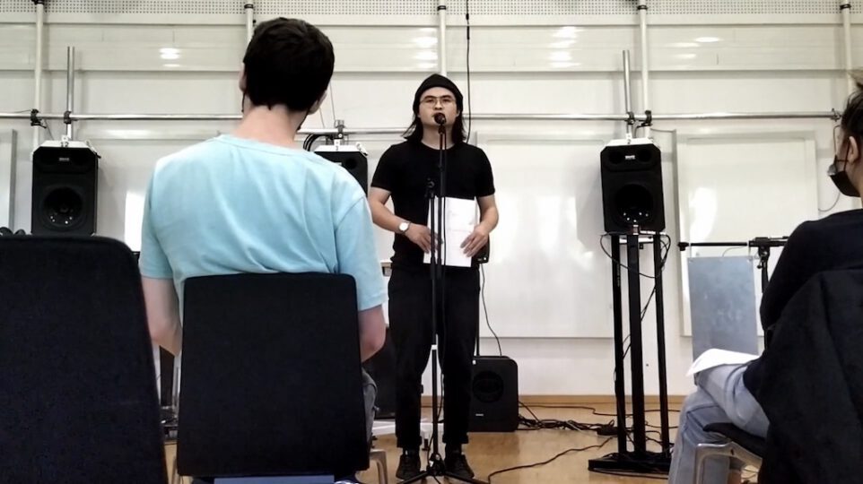
Die grundlegende Idee von maschinellen Lernen lautet „Verbesserung durch Erfahrung“. Der Informatiker Tom M. Mitchell beschreibt es so: „Der Bereich maschinellen Lernen befasst sich mit der Frage, wie man Computerprogramme konstruiert, die sich durch Erfahrung automatisch verbessern.“ (Mitchell, T. (1998). Machine Learning. McGraw-Hill.). Diese Prämisse der „Verbesserung“ hat mich bereits mit nicht-trivialen Fragen konfrontiert. Wenn zum Beispiel maschinelles Lernen eingesetzt wird, um einen improvisierenden Duopartner zu schaffen, was genau versteht der Computer dann als „gute“ oder „schlechte“ Improvisation, wenn er an Erfahrung gewinnt? Das Beantwort dieser ersten Frage ist nötig, bevor man überhaupt mit der Entwicklung eines robusten Algorithmus für maschinelles Lernen beginnen kann. In meinem Stück Shepherd wurde die Elektronik darauf trainiert, meine Stimme zu erkennen, insbesondere ob ich flüstere, rede, schreie oder schweige. Mein Ziel war es jedoch nicht, einen perfekt genauen Erkennungsalgorithmus zu schaffen. Vielmehr wollte ich, dass die Effektivität und die Ineffektivität des Algorithmus bei der Konzeption des Stücks gleiche Wichtigkeit haben. Shepherd ist ein Performance-Stück nach einer Metapher von Jesus aus der christlichen Bibel: Schafe erkennen einen Hirten am Klang seiner Stimme (Johannes 10). Die Elektronik reagiert auf meine Stimme in einer Weise, die gleichzeitig sicher und unsicher ist. Diese Performance ist eine Reflexion über die Nuancen des spirituellen Glaubens, über die Art und Weise, wie Ungewissheit ein notwendige Teil an der Bildung von Überzeugung und Glauben ist. Hier war die Elektronik kein funktionales Instrument (etwas, das von meiner Stimme gesteuert werden sollte), sondern fungierte eher als zweiter Spieler (ein Duopartner, der auf meine Stimme mit einer eingeschränkte Unvorhersehbarkeit reagierte).
Klicken Sie hier für eine deutsche Version dieses Textes.
Up until this past August, my impressions of what machine learning could be used for was mostly functional, detached from any aesthetic reference point within my artistic practice. Cars recognizing stop signs, radiologists detecting malignant legions in tissue; these are the first things to come to my mind. There is definitely an art behind programming these tasks. However, it wasn’t clear to me yet how machine learning could relate to my world of contemporary concert music. Therefore, when I participated in Artemi-Maria Gioti’s machine learning workshop at impuls Academy 2021, my primary interest was to make personal artistic connections to this body of research, and to see what ways I could interrogate my underlying aesthetic assumptions in artistic applications of machine learning. The purpose of this text is to share with you the connections I made. I will walk through the composition process of my piece Shepherd for voice and live electronics, using it as a frame to touch upon basic machine learning theories and methods, as well as outline how I aesthetically reacted to them. I will not go deep into the technicalities of machine learning – there are far more qualified people than I for that specific task. However, I will say that the technical content of this blogpost is inspired heavily from Artemi-Maria Gioti, who led this workshop and whose research covers the creative applications of machine learning in a much deeper way. A further dive into the already rich world of machine learning and music can be begun at her website.
A fundamental definition of machine learning can be framed around the idea of improvement through experience. As computer scientist Tom M. Mitchell describes it, “The field of machine learning is concerned with the question of how to construct computer programs that automatically improve with experience.” (Mitchell, T. (1998). Machine Learning. McGraw-Hill.). This premise of ‘improvement’ already confronted me with non-trivial questions. For example, if machine learning is utilized to create an improvising duo partner, what exactly does the computer understand as ‘good’ or ‘bad’ improvisation, as it gains experience? Before even beginning to build a robust machine learning algorithm, answering this preliminary question is an entire undertaking in and of itself. In my piece Shepherd, the electronics were trained to recognize the sound of my voice, specifically whether I was whispering, talking, yelling, or being silent. However, my goal was not to create a perfectly accurate recognition algorithm. Rather, I wanted the effectiveness and the ineffectiveness of the algorithm to both play equal roles in achieving the piece’s concept. Shepherd is a performance piece takes after a metaphor from Jesus in the christian bible – sheep recognize a shepherd by the sound of their voice (John 10). The electronics reacts to my voice in a way that is simultaneously certain and uncertain. It is a reflection, through performance, on the nuances of spiritual faith, the way uncertainty necessarily partakes in the formation of conviction and belief. Here the electronics were not functional instrument (something designed to be controlled by my voice), but rather were functioning more as a second player (a duo partner, reacting to my voice with a level of unpredictability).
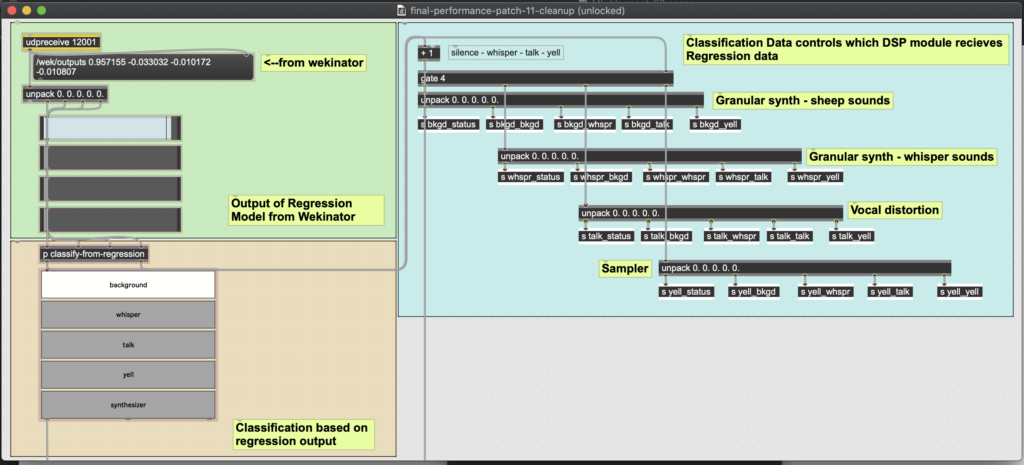
Concretely in the program, the electronics returned two separate answers for every input it is given (see figure 1). It gives a decisive, classification answer (“this is ‘silence’, this is ‘whispering’, this is ‘talking’, etc.), and it gives an indecisive, erratic answer via regression (‘silence: 0.833; whispering: 0.126; talking: 0.201; yelling: 0.044’). And important for this concept of conceiving belief through doubt, the classification answer is derived from the regression answer. The decisive answer (classification) was generally stable in its changes over time, while the indecisive answer (regression) moved more quickly and erratically. Overall, this provided a useful material for creating dynamic control of the actual digital sounds that the electronics produced. But before touching on the DSP, I want to outline how exactly these machine learning algorithms operate, how the electronics learn and evaluate the sound of my voice.
Figure 1: Max MSP and Wekinator (off-screen) analyze an audio’s MFCCs to give two outputs on the nature of the input audio. The first output is from a regression algorithm, the second is from a classification algorithm.
In order for the electronics to evaluate my input voice, it first needs a training set, a collection of data extracted from audio of my voice, with which it could use to ‘learn’ my voice. An important technical point is that the machine learning algorithm never observes actual audio data. With training and testing data, the algorithm is always looking at numerical data (here called ‘descriptors’) extracted from the audio. This is one reason machine learning algorithms can work in realtime, even with audio. As I alluded to, my voice recognition program is underpinned by two machine learning concepts: classification and regression. A classification algorithm will return a discrete value from its input data. In my case, those values are ‘silence’, ‘whispering’, ’talking’, and ‘yelling’. To make a training set then, I recorded audio of each of these classes (4 audio files in total), and extracted MFCCs (Mel-Frequency Cepstrum Coefficients) from it. MFCC’s are a representation a sound’s spectral energy calibrated to the range of typical human auditory perception, and are already commonly used in speech recognition programs, music-information retrieval applications, and other applications based around timbre-recognition.
I used the Max MSP library Zsa.descriptors to calculate my MFCCs. I also experimented with other audio descriptors such as spectral centroid, spectral flatness, amplitude peaks, as well as varying numbers of MFCC’s. Eventually I discovered that my algorithm was most accurate when 13 MFCCs were the only descriptor, and that description data was taken only about fivetimes a second. I realized that, on a micro-level timescale, my four classes had a lot similarity. For example, the word ‘synthesizer,’ carried lots of ’s’ noise, which is virtually the same when whispered as when talked. Because of this, extracting data at an intentionally slower rate gave the algorithm a more general picture of each of my voice-classes, allowing these micro-moments of similarity to be smoothed out.
The standard algorithm used for my voice recognition concept was classification. However, my classification algorithm was actually built using a second common machine learning algorithm: regression. As I mentioned before, I wanted to build into my electronics a level of ‘indecision’, something erratic that would contrast the stable nature of a standard classification algorithm. Rather than returning discrete values, a regression algorithm gives a new ‘predictive’ value, based on a function derived from the training set data. In the context of my piece, the regression algorithm does not return a specific voice-class. Rather, it gives four percentage values, each corresponding to how close or far my input is to each of the four voice-classes. Therefore, though I may be whispering, the algorithm does not say whether I am whispering or not. It merely tells me how close or far away I am from the ‘whispering’ data that it has been trained on.
I used a regression algorithm in Wekinator, a simple and powerful machine learning tool, to build my model (see figure 2). Input audio was analyzed in Max MSP, and the descriptor data was sent via OSC to Wekinator. Wekinator built the predictive regression model from this data and then sent output back to Max MSP to be used for DSP control. In Max, I made my own version of a classification algorithm based on this regression data.
Figure 2: Wekinator is evaluating MFCC data from Max MSP and returning 4 values from 0.0-1.0, indicating the input’s similarity to the four voice classes (silence, whispering, talking, yelling). The evaluation is a regression model trained on 752 data samples.
All this algorithm-building once again returns me to my original concern. How can I make an aesthetic connection with these concepts? As I mentioned, this piece, Shepherd is for my solo voice and live electronics. In the piece I stand alone on a stage, switching through different fictional personas (a speaker at a farming convention, a disgruntled restaurant chef, a compilation video of Danny Wolfers saying the word ‘synthesizer,’ and a preacher), and the electronics reacts to these different characters by switching through its own set of personas (sheep; a whispering, whimpering sous chef; a literal synthesizer; and a compilation of christian music). Both the electronics and I change our personas in reaction to each other. I exercise some level control over the electronics, but not total. As I said earlier, the performance of the piece is a reflection on the intertwinement of conviction and doubt, decision and indecision, within spiritual faith. Within this concept, the idea of a machine ‘improving’ towards ‘perfection’ is no longer an effective framework. In the concept, and consequently in the music I attempted to make, stable belief (classification) and unstable indecision (regression) were equal contributors towards the musical relationship between myself and the electronics.
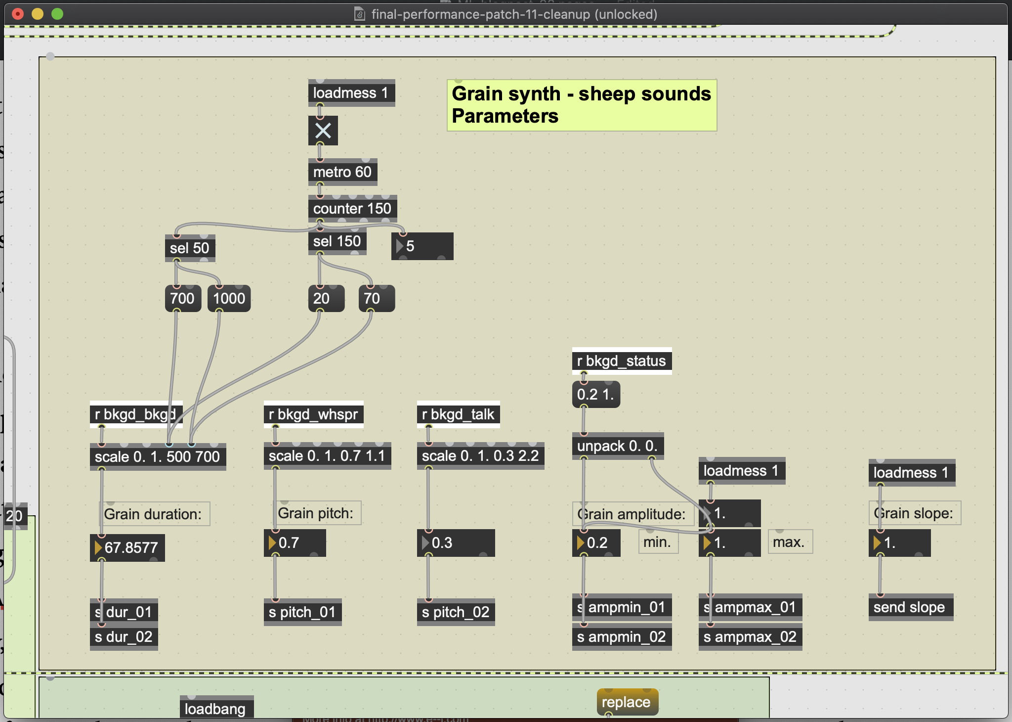
Based on how my voice was classified, the electronics operated one of four DSP modules. The individual parameters of a given module were controlled by the erratic output data of the regression algorithm (see figure 3). For example, when my voice was classified as silent, a granular synthesizer would create textures of sheep-like noises. Within that synthesizer, the percentage levels of whispering and talking ‘detected’ within the silence would manipulate the pitch shifting in the synthesizer (see figure 4). In this way, the music was not just four distinct sound modules. The regression algorithm allowed for each module to bend and flex in certain directions, as my voice subtly suggested hints of one voice class from within another. For example, in one section I alternate rapidly between the persona of a farmer talking at a farming convention, and a chef frustratingly whispering at his sous chef. The electronics moved consequently between my whispering and talking DSP modules. But also, as my whispering became more frustrated and exasperated, the electronics would output higher levels of talking in its regression algorithm. Thus, the internal drama of my theatricalperformances is reacted to by the electronics.
Figure 3: The classification data would trigger one of four DSP modules. A given DSP module would receive the regression values for all four vocal classes. These four values would control the parameters of the DSP module.
Figure 4: Parameter window for granular synth triggered when the electronics classifies my voice as ‘silent’. The amount of whispering and talking detected in the silence would control the pitch of the grain. The amount of silence detected in the silence controlled the grain’s duration. Because this value is relatively static during actual silence from my voice, a level of artificial duration manipulation (seen a the top of the window) was programmed.
I want to return to Tom Mitchell’s thesis that machine learning involves computer improvingautomatically through experience. If Shepherd is a voice recognition tool, then it is inefficient at improvement. However, Shepherd was not conceived as a tool. Rather, creating Shepherd was more so a cultivation of a relationship between my voice and the electronics. The electronics were more of a duo partner, and less of an instrument. To put this more concretely, I was never looking for ‘accurate’ results from the machine. As I programmed, I was searching for results that illustrated Shepherd’s artistic concept of belief intertwined with doubt. In this way, ‘improving’ the piece did not mean improving the algorithm’s accuracy. It meant ‘improving‘ the relationship between myself and the electronics. One positive from this approach is that the compositional process was never separated from the programming of the electronics. Both developed in tandem. The composing this piece brought me to the realization that creative applications of machine learning can be applied at every level of its discourse. If you ware interested in hearing a recording of this performance, a bootleg recording of the premiere can be found here.
References:
Artemi-Maria Gioti – composer and artistic researcher working in the field of artificial intelligence.
Wekinator – free, open-source software created by Rebecca Fiebrink that uses machine learning to create musical instruments, game interfaces, computervision, and other tools in sound and animation.
Zsa.descriptors – library for real-time sound descriptors analysis for Max MSP developed by Mikhail Malt and Emmanuel Jourdan.