Texture Synthesis: Overview
The second application is a texture synthesis tool that uses an unsupervised clustering algorithm to group a set of audio files according to a combination of several audio descriptors. Texture synthesis is referred to in this context as the reconstitution of certain sound characteristics via smaller preexisting sound elements.
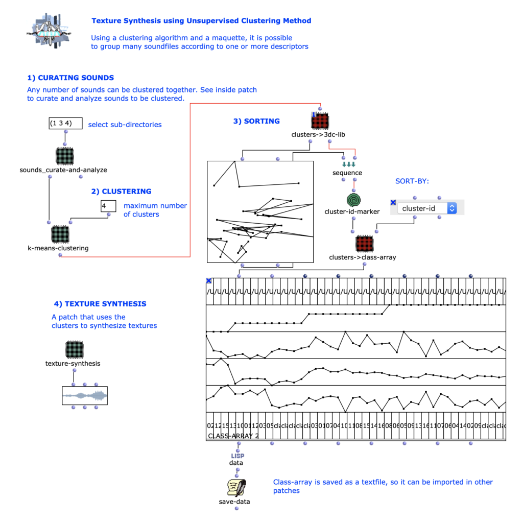
Figure 10: Overview of the Texture Synthesis application.
Each sound in this library is analyzed and converted to a vector containing the filepath, its audio descriptors (spectral centroid, spectral difference, and covariance) and its cluster group-id. This information is represented in a class array object (see figure 12), where it can also be sorted by any one of the vector’s values. The power of the cluster algorithm is that it condenses all of a vector’s descriptor values into a single value, from which is groups similar sounds into clusters. This means that sorting by cluster-id is a way of relating sounds to each other in a multi-dimensional (i.e. multiple parameters) way.
Audio V is an example of texture synthesis from the patch. It uses a combination of automated and hand-placed sound concatenation (see figure 11).
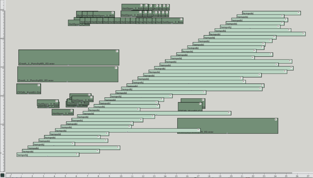
Figure 11: The cluster-sorted automated texture synthesis are the light green temporal objects. The dark green sounds were hand-placed in the maquette.
The automated portion of the texture synthesis is organized such that a library of clarinet, saxophone, and violin sounds are simply played one after another, sorted according to cluster-id. This sorting can be seen in Figure 15, which is a class array representing all the data from each audio vector. The first six sounds in Audio V make up the first cluster group. The next 11 sounds make up the second group, and the last 24 sounds make up the final, third group. Figure 13 is another way of visualizing the cluster groups, via a 3DC-library.
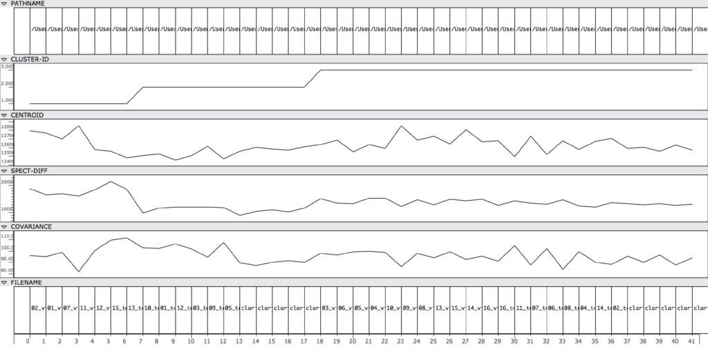
Figure 12: The first six sounds are clustered into a single group, while the next 11 sounds are in a second group. The remaining 24 sounds are in group 3.
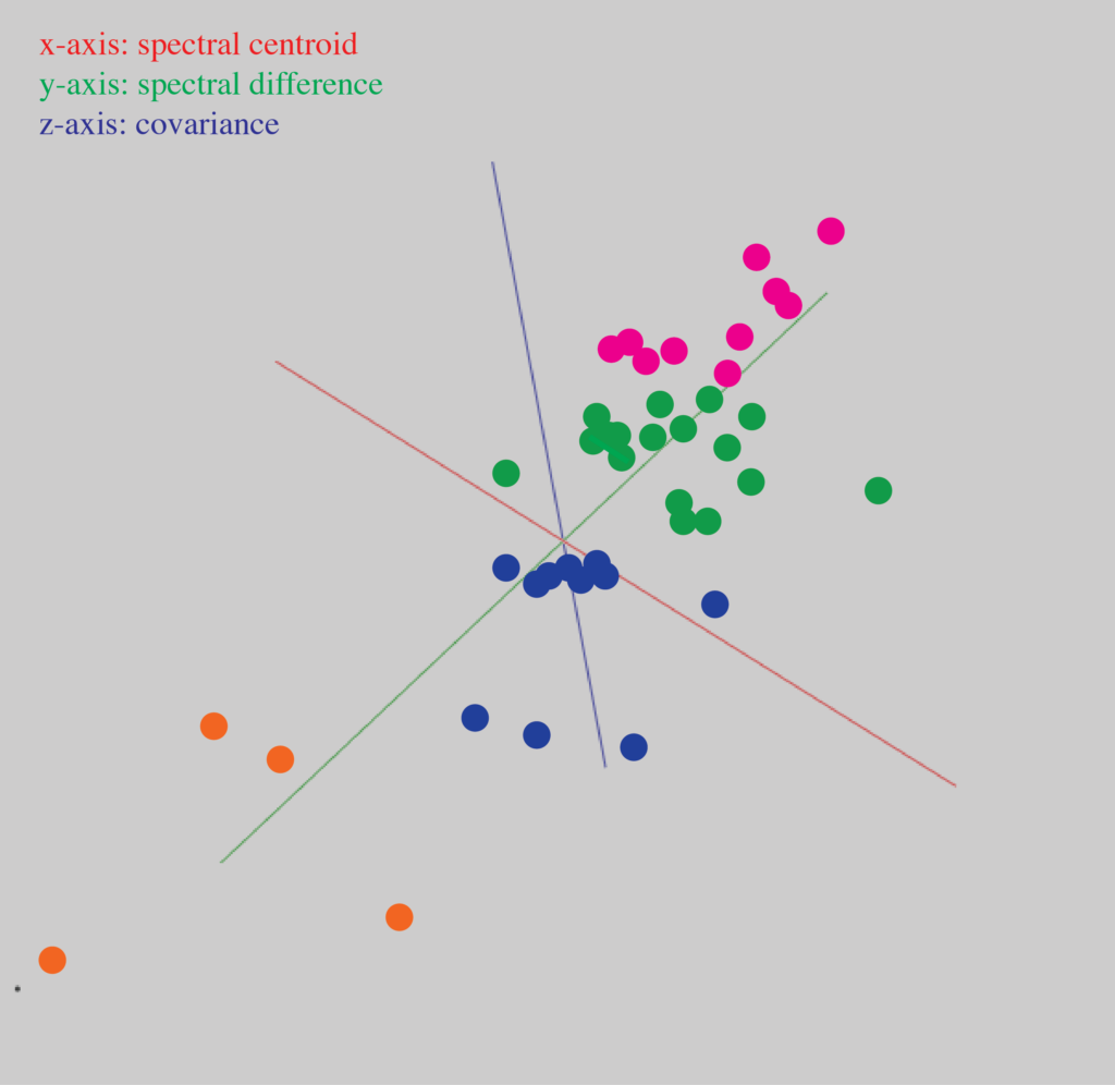
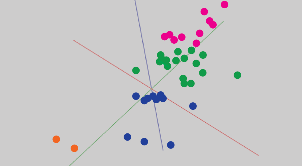
Figure 13: The input audio is represented in 3d space, where it is possible to see specific relationships between each sounds audio descriptors.
Note that though there are three different instruments amongst the entire audio library used for figure 13, the cluster groups did not simply align according to instrumental type. For example, cluster-group 1 contained both violin and tenor saxophone sounds.
Texture Synthesis: Clustering Method
A simple k-means clustering algorithm is used to group the input sounds. Like the k-nearest neighbors algorithm, we can visualize a k-means clustering algorithm on a graph with each point representing an input sound. However, unliked the supervised method of classification, there is no training set data. The algorithm seeks to find similarities amongst the input data, rather than comparing it to an external training set (see figure 14).
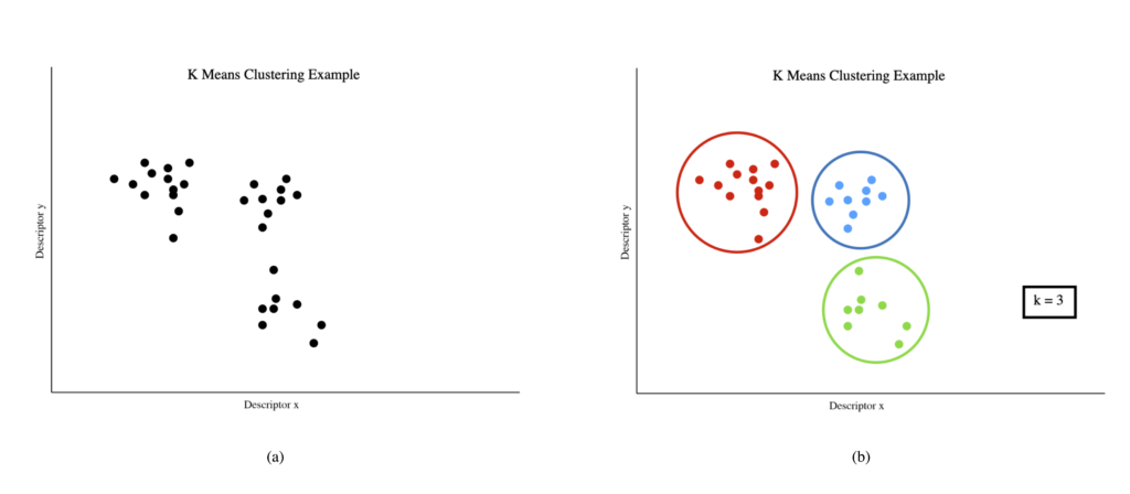
Figure 14: A set of data before (a) and after (b) it has been clustered by a 3 mean clustering algorithm
A ’mean’ in this context refers to the ‚centroid‘ of a given cluster. Thus, a 3-mean clustering algorithm will return 3 clusters. First, a number (k) of random ’means’ are generated. Each data point then is grouped with the ‚mean‘ that it is closest to. For our k = 3 example, this means that there are now three clusters of sounds. However, these sounds are clustered around a randomly generated mean. It is not the actual centroid of the cluster. Thus the second step is to calculate the actual centroid of each of these clusters. From here, the first and second step are repeated again – each data point is regrouped to be with the closest of the three new centroids that were calculated in step 2, created another set of 3 clusters. Step 2 is repeated with these new clusters, and the overall process is repeated until the centroids cease to change between iterations.
Downloading and Using the Applications
These two applications can be downloaded in the form of OpenMusic patches in this link above. Due to copyright purposes, the audio used in the examples and training set cannot be distributed with the patches.
References
- R. Bittner, J. Wilkins, H. Yip, J. Bello, „MedleyDB 2.0: New Data and a System for Sustainable Data Collection.“ New York, NY, USA: International Conference on Music Information Retrieval, 2016 – An annotated open source dataset for music information retrieval.
- D. Schwarz, “State of the Art in Sound Texture Synthesis,” in International Conference on Digital Audio Effects, Paris, France, 2011.
- A. Vinjar, “OMAI: An AI Toolkit For OM#,” in Linux Audio Conference, Bordeaux, France, 11 2020.
- B. Hackbarth, N. Schnell, and D. Schwarz, “Audioguide: a Framework for Creative Exploration of Concatenative Sound Synthesis,” Tech. Rep., Mar. 2011.
- M. Malt, E. Jourdan, „Zsa.Descriptors: a library for real-time descriptors analysis.“ in 5th Sound and Music Computing Conference, Berlin, Germany, Jul 2008, Berlin, Germany. pp.134-137.
- M. Schumacher, OM-Pursuit – a library for dictionary-based sound analysis/synthesis methods in OpenMusic.
Über den Autor