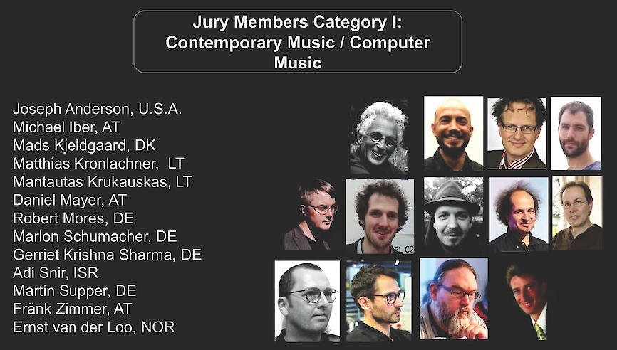
In October 2022, I served as a jury member for the Student 3D Audio production Competition from the Verband Deutscher Tonmeister e.V. The competition comprised of 3 categories. I was a judge in the category Contemporary Music/Computer Music.
The winning productions can be listened to online via head-tracked binaural audio, using this excellent (computervision-based) web-audio player here.
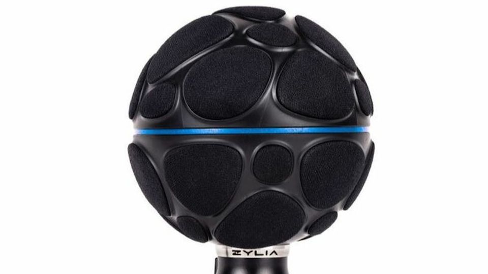
Abstract: Beschreibung des 6DOF Recording Systems der Firma Zylia für HOA und dessen Software, mit Streaming und Binauralix Anwendungen.
Verantwortliche: Prof. Dr. Marlon Schumacher, Eveline Vervliet
Introduction
The Zylia microphone is a 19-capsule microphone array used for 3D/360 audio recording in 3rd ambisonics order. It’s easy to connect to your computer with a USB cable and compact in transportation.
Software
For proper functioning of the Zylia ZM-1, you must install a driver. Download the driver specific for your operating system here.
Zylia 6DoF Recording Application for recording with multiple Zylia microphones Zylia Ambisonics Converter for converting from A to B format Zylia Control Panel with some information on the connected microphone Zylia Streaming Application for setting up your live audio streaming with the Zylia microphone Zylia Studio for recording with one Zylia microphone
Download the software here. Note that licenses are required.
Workflow
Recording
Recording with the Zylia microphone can be done either in the standalone application Zylia Studio or in a DAW with the Zylia Studio Pro audio plugin. As a DAW, Reaper is most recommended.
Conversion
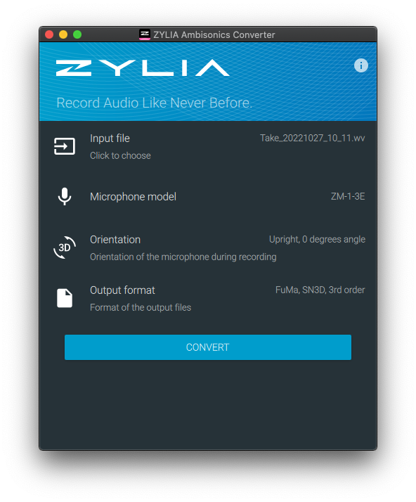
To use the recordings on other platforms or for applications like videos, the recordings have to be converted to an Ambisonics B-format. You can either use the standalone application or the Zylia Ambisonics Converter plugin.
There are several standards in the ambisonics world related to channel ordering and normalization levels. The most used one is the ambiX standard. For this, you choose the following settings: channel ordering ‚ACN‘ and normalization ‚SN3D‘. The following video from ZYLIA explains the workflow for converting a recording.
The raw recording from the Zylia microphone will contain of 19 channels. The converted file in B-format in 3rd order will have 16 channels. First encode the B-format in a software like MultiPlayer-mini before integrating it with the open-source software Binauralix.
In the following demonstration video, I open the 3rd order B-format of a Zylia recording in multiplayer mini and send it to Binauralix over Blackhole. The I communicate with Binauralix over OSC in Max. In this way, I can use the BITalino R-IoT sensor to control the listening orientation in Binauralix in real-time.
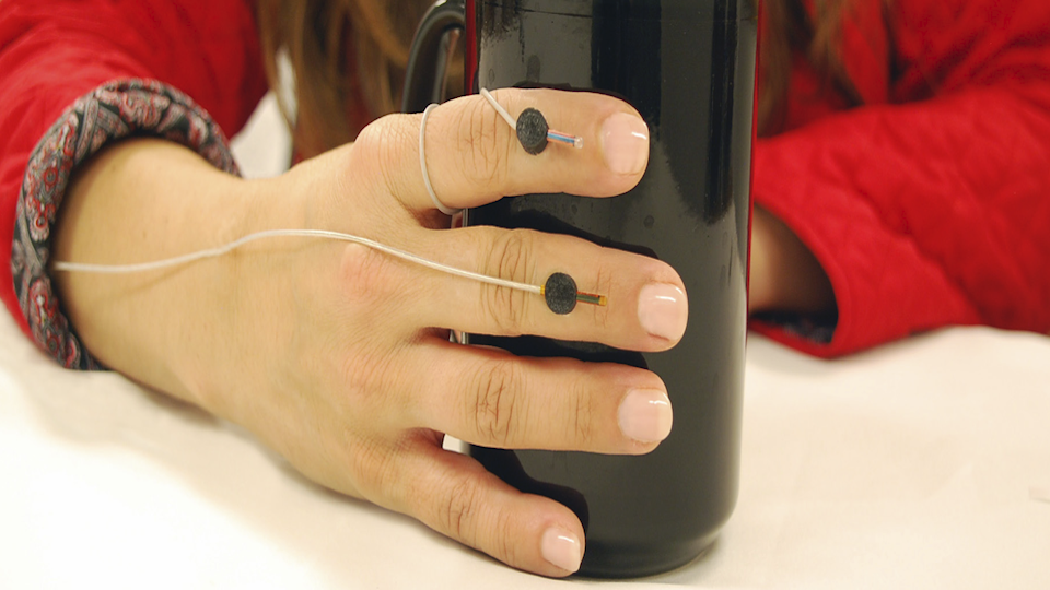
Abstract: Beschreibung des Inertial Motion Tracking Systems Bitalino R-IoT und dessen Software
Verantwortliche: Prof. Dr. Marlon Schumacher, Eveline Vervliet
Introduction
In this blog, I will explain how we can use machine learning techniques to recognize specific conductor gestures sensed via the the BITalino R-IoT platform in Max. The goal of this article is to enable you to create an interactive electronic composition for a conductor in Max.
This project is based on research by Tommi Ilmonen and Tapio Takala. Their article ‚Conductor Following with Artificial Neural Networks‘ can be downloaded here. This article can be an important lead in further development of this project.
Demonstration Patches
In the following demonstration patches, I have build further on the example patches from the previous blog post, which are based on Ircam’s examples. To detect conductor’s gestures, we need to use two sensors, one for each hand. You then have the choice to train the gestures with both hands combined or to train a model for each hand separately.
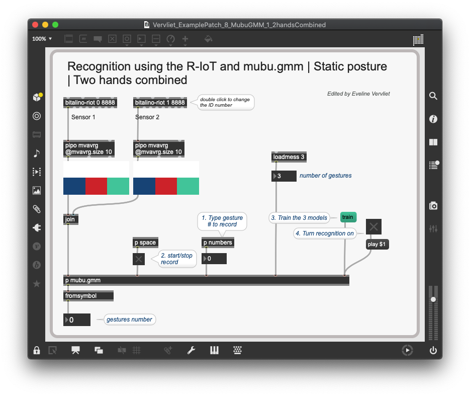
Detect static gestures with 2 hands combined
When training both hands combined, there are only a few changes we need to make to the patches for one hand.
First of all, we need a second [bitalino-riot] object. You can double click on the object to change the ID. Most likely, you’ll have chosen sensor 1 with ID 0 and sensor 2 with ID 1. The data from both sensors are joined in one list.
In the [p mubu.gmm] subpatch, you will have to change the @matrixcols parameter of the [mubu.record] object depending on the amount of values in the list. In the example, two accelerometer data lists with each 3 values were joined, thus we need 6 columns.
The rest of the process is exactly the same as in previous patches: we need to record two or more different static postures, train the model, and then click play to start the gesture detection.
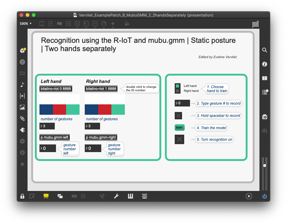
When training both hands separately, the training process becomes a bit more complex, although most steps remain the same. Now, there is a unique model for each hand, which has to be trained separately. You can see the models in the [p mubu.gmm-left] and [p mubu.gmm-right] subpatches. There is a switch object which routes the training data to the correct model.
In the above example, I personally found the training with both hands separate to be most efficient: even though the training process took slightly longer, the programming after that was much easier. Depending on your situation, you will have to decide which patch makes most sense to use. Experimentation can be a useful tool in determining this.
Detect dynamic gestures with 2 hands
The detection with both hands of dynamic gestures follow the same principles as the above examples. You can download the two Max patches here:
The mentioned tools can be used to detect ancillary gestures in musicians in real-time, which in turn could have an impact on a musical composition or improvisation. Ancillary gestures are „musician’s performance movements which are not directly related to the production or sustain of the sound“ (Lähdeoja et al.) but are believed to have an impact both in the sound production as well as in the perceived performative aspects. Wanderley also refers to this as ‘non-obvious performer gestures’.
In a following article, Marlon Schumacher worked with Wanderley on a framework for integrating gestures in computer-aided composition. The result is the Open Music library OM-Geste. This article is a helpful example of how the data can be used artistically.
Links to articles:
Marcelo M. Wanderley – Non-obvious Performer Gestures in Instrumental Musicdownload
O. Lähdeoja, M. M. Wanderley, J. Malloch – Instrument Augmentation using Ancillary Gestures for Subtle Sonic Effectsdownload
M. Schumacher, M. Wanderley – Integrating gesture data in computer-aided composition: A framework for representation, processing and mappingdownload
Detecting gestures in musicians has been a much-researched topic in the last decades. This folder holds several other articles on this topic that could interest.
Abstract: Beschreibung des Inertial Motion Tracking Systems BITalino R-IoT und dessen Software
Verantwortliche: Prof. Dr. Marlon Schumacher, Eveline Vervliet
Introduction to the BITalino R-IoT sensor
The R-IoT module (IoT stands for Internet of Things) from BITalino includes several sensors to calculate the position and orientation of the board in space. It can be used for an array of artistic applications, most notably for gesture capturing in the performative arts. The sensor’s data is sent over WiFi and can be captured with the OSC protocol.
The R-IoT sensor outputs the following data:
Accelerometer data (3-axis)
Gyroscope data (3-axis)
Magnetometer data (3-axis)
Temperature of the sensor
Quaternions (4-axis)
Euler angles (3-axis)
Switch button (0/1)
Battery voltage
Sampling period
The accelerometer measures the sensor’s acceleration on the x, y and z axis. The gyroscope measures the sensor’s deviation from its ’neutral‘ position. The magnetometer measures the sensor’s relative orientation to the earth’s magnetic field. Euler angles and quaternions measure the rotation of the sensor.
The sensor has been explored and used by the {Sound Music Movement} department of Ircam. They have distributed several example patches to receive and use data from the R-IoT sensor in Max. The example patches mentioned in this article are based on these.
The sensor can be used with all programs that can receive OSC data, like Max and Open Music.
Max patches by Ircam and other software software/ ├motion-analysis-max-master/ │├max-bitalino-riot/ ││⎿bitalino-riot-analysis-example.maxpat │├max-motion-features/ ││├freefall.maxpat ││├intensity.maxpat ││├kick.maxpat ││├shake.maxpat ││├spin.maxpat ││⎿still.maxpat │ ⎿README.md
Demonstration Videos
In the following demonstration videos and example patches, we use the Mubu library in Max from Ircam to record gestures with the sensor, visualise the data and train a machine learning algorithm to detect distinct postures. The ‚Mubu for Max‘ library must be downloaded in the max package manager.
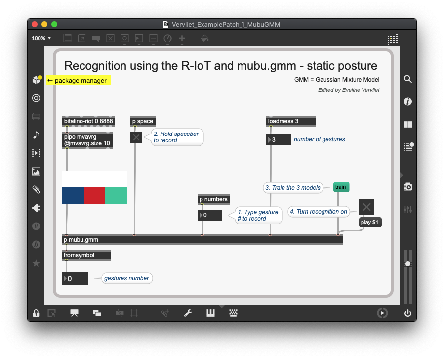
Detect static gestures with mubu.gmm
First, we use the GMM (Gaussian mixture model) with the [mubu.gmm] object. This model is used to detect static gestures. We use the accelerometer data to record three different hand postures.
Detect dynamic gestures with Mubu Gesture Follower
The Gesture Follower (GF) is a separate tool from the Mubu library that can be used in gesture recognition applications. In the following video, the same movements are trained as in the Mubu.hhmm demonstration so we can easily compare both methods.
Gesture detection and vocalization with Mubu in Max for the Bitalino R-IoT
The [mubu.xmm] object uses hierarchical multimodel hidden Markov models for gesture recognition. In the following demonstration video, gestures and audio is recorded simultaneously. After training, a gesture will trigger its accompanying audio recording. The sound is played back via granular or concatenative synthesis.
Abstract: Der Eintrag beschreibt die Spatialisierung des Stückes »Ode An Die Reparatur« (2021) und dessen Transformation in eine Higher Order Ambisonics Version. Ein binauraler Mix des fertigen Stückes ermöglicht es, den Arbeitsprozess anhand des Ergebnisses nachzuvollziehen.
Betreuer: Prof. Dr. Marlon Schumacher
Ein Beitrag von: Jakob Schreiber
Stück
Das Stück »Ode An Die Reparatur« (2021) besteht aus vier Sätzen, von denen jeder sich auf einen anderen Aspekt einer fiktiven Maschine bezieht. Interessant an diesem Prozess war es, den Übergang von Maschinenklängen in musikalische Klänge zu untersuchen und über den Verlauf des Stückes zu gestalten.
Produktion
Die Produktions-Ressourcen des Stückes waren einerseits ein UHER-Tonbandgerät, welches einfache Repitch-Veränderungen ermöglicht und durch seine Funktionsweise mit Motoren und Riemen für die Umsetzung dieses an mechanische Maschinen angelehnten Stückes prädestiniert war. Außerdem kam SuperCollider als digitale Klangsynthese- und Verfremdungsumgebung zum Einsatz.
Aufbau
Das Stück besteht aus vier Sätzen.
Erster Satz
Das Tonmaterial des Beginns setzt sich aus verschiedenen Aufnahmen eines Tonbandgerätes zusammen, über welches neben Stille klar hörbare, synthetisierte Motoren-Klänge abgespielt werden.
Zweiter Satz
Die zu manchen Teilen an Vogelgezwitscher erinnernden Klangobjekte treten teils unvermittelt aus steriler Stille in den Vordergrund.
Dritter Satz
Die perforative Charakteristik im inneren eines Zahnradgetriebes transformiert sich im Verlauf des Satzes zu tonal ausgebildeten Resonanzen.
Vierter Satz
Im letzten Satz spielen die Motoren eine monumental anmutende Abschluss-Hymne.
Spatialisierung
Angelehnt an die kompositorische Form des Stückes halten sich die Spatialisierungs-Entwürfe an die Unterteilung in Sätze.
Arbeits-Praxis
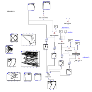
Der Arbeitsprozess lässt sich, ähnlich wie der OM-Patch, in verschiedene Bereiche aufteilen. Im Labor-Abschnitt erforschte ich verschiedene Spatialisierungsformen auf ihre Ästhetische Wirkung hin und untersuchte deren Übereinstimmung mit der kompositorischen Form des bereits bestehenden Stückes.
Um verschiedene Trajektorien, oder feste Positionen von Klangobjekten zu ermitteln spielte neben der auditiven Wirkung auch die visuelle Einschätzung der jeweiligen Trajektorien eine wichtige Rolle.
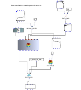
Letztendlich wurden die Paramter der bereits vorausgewählten Trajektorien mit einem Streuungsverlauf ergänzt, fein justiert und schließlich über eine Kette aus Modulen in ein Higher Order Ambisonics Audiofile fünfter Ordnung transformiert.
In Iterativer Weise werden die synthetisierten Mehrkanal-Dateien in REAPER in das Gesamtgefüge eingepflegt und deren Wirkung untersucht, bevor sie mit einem optimierten Set an Parametern und Trajektorien noch einmal den Syntheseprozess durchlaufen.
Näheres zu den einzelnen Sätzen
Zunächst kann hier die binaurale Version des spatialisierten Stückes als ganzes angehört werden. In der Folge werden kurz die Herangehensweisen der einzelnen Teile beschrieben
Erster Satz
Die lange gezogenen, wie Schichten übereinander liegenden Klanwolken bewegen sich im ersten Teil dem Grundtempo des Satzes entsprechend. Die Trajektorien liegen dabei in der Summe U-förmig um den Hör-Bereich, wobei sie nur die Seiten und Vorderseite abdecken.
Zweiter Satz
Einzelne Klang-Objekte sollen aus sehr verschiedenen Positionen zu hören sein. Nahezu perkussive Klänge aus allen Richtungen des Raumes lassen die Aufmerksamkeit der Hörer*in springen.
Dritter Satz
Das klangliche Material des Teiles ist eine an den Klang von Zahnrädern, oder eines Getriebes angelehnte Klangsynthese. Das Augenmerk hierbei lag in der Immersion in die fiktive Maschine. Aus eben diesem Klangmaterial entstehen durch Resonanzen und andere Veränderungen liegetöne, die sich zu kurzen Motiven aneinander reihen.
Das Spatialisierungskonzept für diesen Teil setzt sich aus beweglichen und teilweise statischen Objekten Zusammen. Die beweglichen erschaffen zu Beginn des Satzes eine Anmutung von Räumlichkeit Immersion. Zum Ende des Satzes kommen zwei verhätnismäßig statische Objekte links und rechts der Stereobasis hinzu, die vor allem die melodie-haften Aspekte des Klanges hervorheben und an ihrer jeweiligen Position lediglich flüchtig auf der vertikalen Achse oszillieren.
Vierter Satz
Die Instrumentierung dieses Teiles des Stückes setzt sich aus drei Simulationen eines Elektromotors zusammen, die jeweils eine Eigene Stimme verfolgen. Um die einzelnen Stimmen noch etwas besser voneinander zu trennen, entschied ich mich dazu, jeden der vier Motoren als einzelnes Klangobjekt zu behandeln. Um den monumentalen Charakter des Schlussteils zu unterstützen, bewegen sich die Objekte dabei nur sehr langsam durch den fiktiven Raum.
In diesem umfassenden Artikel werde ich den Schaffensprozess meiner Komposition beschreiben, um meine Erfahrung im Zuge der Mehrkanal-Bearbeitungen zu präsentieren. Die Komposition habe ich im Rahmen des Seminars „Visuelle Programmierung der Raum/ Klangsynthese (VPRS)“ bei Prof. Dr. Marlon Schumacher an der HFM Karlsruhe produziert.
Betreuer:: Prof. Dr. Marlon Schumacher Eine Studie von: Mila Grishkova
Somersemester 2022
Hochschule für Musik, Karlsruhe
✅ Das Ziel
Das Ziel meiner Projektarbeit war es, eine komplette Erfahrung mit der Mehrkanal-Bearbeitung zu bekommen.
Ich benutze 3 Klänge um Komposition zu bauen.
Dann realisiere ich das Stück im Format 3D Ambisonics 5. Ordnung (36-Kanal Audiodatei). Ich benutze Mehrkanal-Bearbeitungen mit OM-SoX Spatialisierung/Rendering in Ambisonics mit OMPrisma, hierbei: Dynamische Spatialisierung (hoa.continuous). Die resultierenden Audio Dateien importiere ich in ein entsprechendes Reaper Projekt (Template wird zur Verfügung gestellt (s. Fig 7)). Innerhalb Reaper sind die Ambisonics Audiospuren mit Plugins bearbeitet.
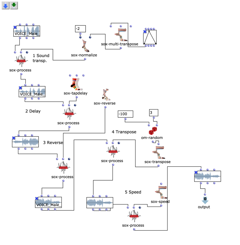
✅ 1. Figur & 1. Sound
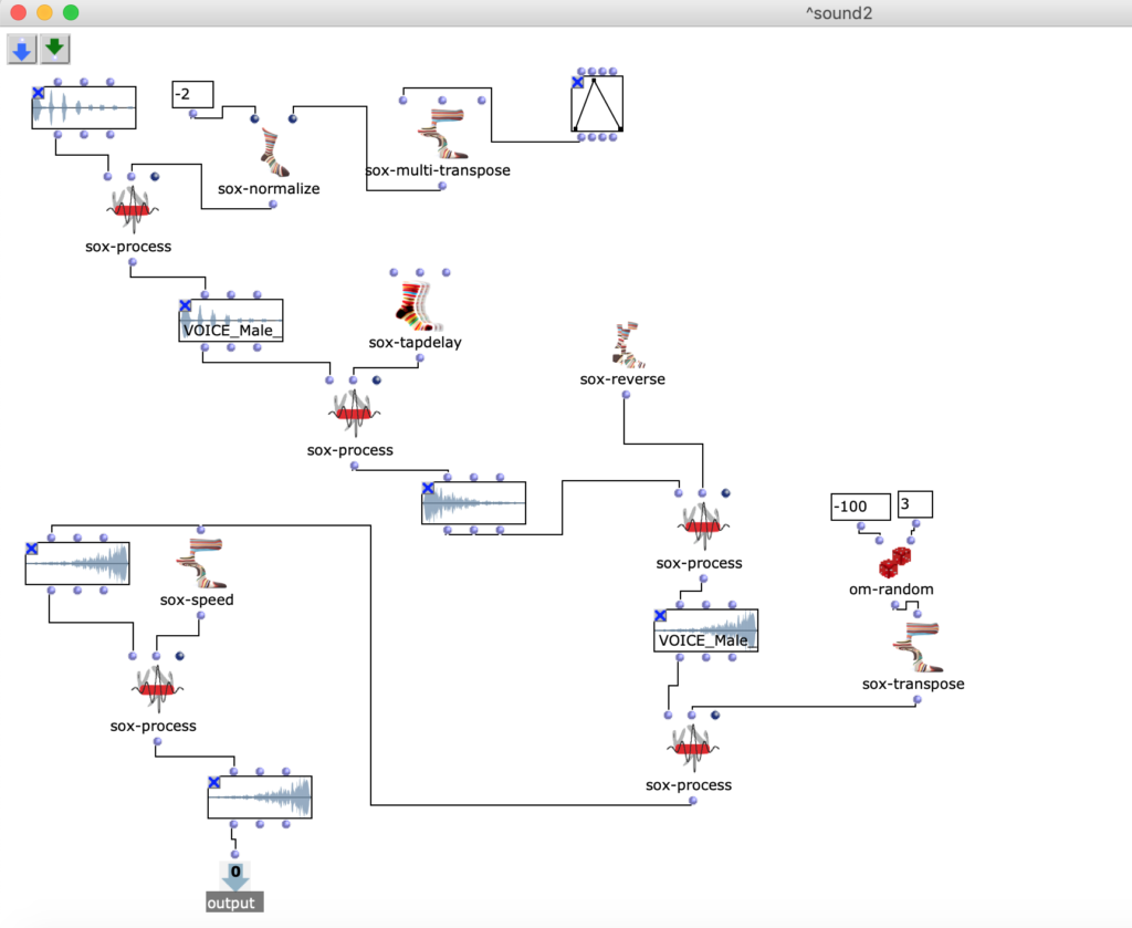
In der 1. Figur kann man einen OpenMusik Patch erkennen. In dem Patch „Sound1“ befindet sich die Methode Sound1 zum bearbeiten. Ich benutze Sound-voice, dann mache ich eine Transposition (OMsox-transpose, OM sox-normalize), dann benutze ich Verzögerungsleitungen (OMsox-tapdelay). Nächster Schritt ist rückwärts (OM sox-reverse). Dann kann man in Patch Transposition sehen und ich benutze die random-Methode (OM sox-random). Das letzte Element dieses Patches ist die Speed-Bearbeitung (OM sox-speed).
Fg. 1 zeigt OpenMusic Patch Sound1: Dieser Patch zeigt transformation des 1.Sounds
In der 2. Figur kann man einen OpenMusik Patch sehen. In dem Patch „Sound2“ befindet sich die Methode „Sound2“ zum bearbeiten. Ich mache die gleiche Manipulationen, wie mit dem 1. Sound, um 2.Sound zu bearbeiten. Die Beschreibung kann man oben lesen.
Fg. 2 zeigt OpenMusic Patch Sound2: Dieser Patch zeigt transformation des 2.Sounds
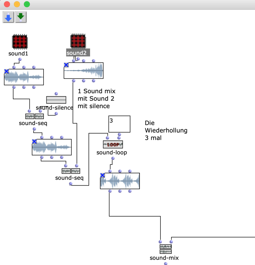
In der 3. Figur kann man den OpenMusic Patch „Mix“ sehen. In diesem Patch befindet sich der MixProzess „2 Klänge“ (OM sound-mix), die ich in den letzten 2 Patches beschrieben habe. Ich addiere Pausen (OM sound-silence) und dann wiederhole ich das Klangmaterial 3 mal (OM sound-loop).
Fg. 3 zeigt OpenMusic Patch „Mix“: Dieser Patch zeigt Sound-mix (Sound 1 und Sound 2).
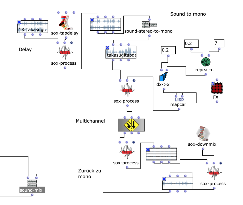
In der 4. Figur befindet sich der Patch 4, in dem man die Bearbeitung der Komposition von Takasugi „Diary of a Lung“ sehen kann.
Der Komponist Steven Kazuo Takasugi hat seine Musikstuck „Diary of a Lung, version for eighteen musicians and electronic playback“ an der Hochschule für Musik Karlsruhe präsentiert und er hat 2 Toningenieure gesucht, die seine Komposition bei dem Konzert live mit mehreren Kanäle abspielen können.
„Takasugi ist heute einer der renommiertesten Komponisten im Bereich Neue Musik. Seine Arbeit konzentriert sich auf elektroakustische Komposition, meist mit musiktheatralischen Elementen: Sein international gefeiertes Werk „Sideshow“ für Live-Oktett, elektronische Verstärkung und Wiedergabe (2009–2015) ist ein gutes Beispiel. Bemerkenswerterweise umfasst sein Œuvre weniger als zwei Dutzend Werke. Oft arbeitet er jahrelang an einem Stück – umso größer ist die Spannung, mit der jedes neue Stück erwartet wird.“(C)
Herr Takasugi entwickelt seine Musiksprache. Als Komponist, hat Herr Takasugi hat seine Komposition mit einer Konzeption verarbeiten. Die Hauptidee war, dass man muss seinen Körper als ein Instrument benutzen. Takasugis Projekte zeichnen sich durch eine Bezugnahme nicht nur auf den Inhalt des künstlerischen Ausdrucks (zum Beispiel den Inhalt eines musikalischen Werks), sondern auch auf den Ausdrucksakt (die Tatsache, dass Musik gespielt wird, den Körper des Interpreten, der Atem des Darstellers).
Körperkonzept spielt eine große Rolle in Takasugis Philosophie. Der Körper bringt in dem Prozess die Zeit und hilft in dem Moment (hier und jetzt) sich zu fokussieren. Der Körper hilft, diesen Prozess als meditativen Prozess wahrzunehmen. Um dieses Musikstuck zu produzieren, hat Herr Tahasugi sich und verschiedene Klänge von seinem Körper aufgenommen.
Die Tonregie muss große Verantwortung übernehmen und muss als Instrumentalist die Musik abspielen. Deswegen können diese Arbeit, das Audiosignal an mehrere Kanäle zu schicken, weder eine Machine noch Computer oder Code (lautet Herr Takasugi) übernehmen.
Als Tonregie habe ich dieses Musikstuck gespielt. Genau deswegen war es für mich (als Musikinformatikerin) interessant zu testen, was man in dieser Musik algorithmisieren kann.
Deswegen, habe ich als Teil meines Materials Takasugi’s Musikstuck genommen.
Als Bearbeitungsmethode benutze ich delay (OM sox-tapdelay), dann mache Stereo zu Mono. In Patch „FX“ befinden sich OM sox-phaser, OM sox-tremolo (s. Fg 5).
Fg. 4 zeigt OpenMusic Patch „Takasugi“: Dieser Patch zeigt Bearbeitung des Materials vom Audio Takasugi „Diary of a Lung“
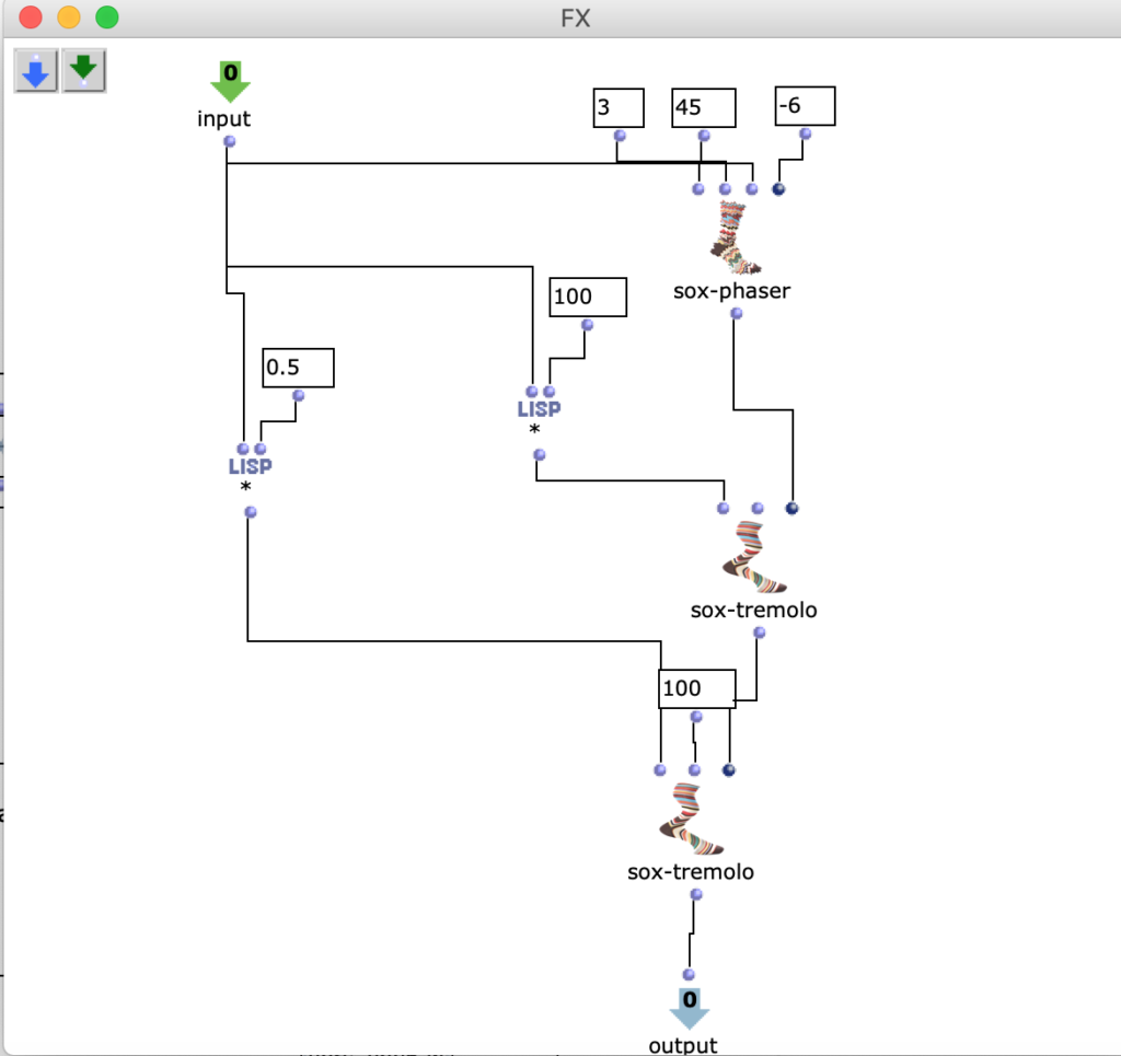
In der nächsten Figur (Fig. 5) kann man den Patch „FX“ sehen.
Fg. 5 zeigt OpenMusic Patch „FX“: Dieser Patch zeigt OM sox-phaser, OM sox-tremolo
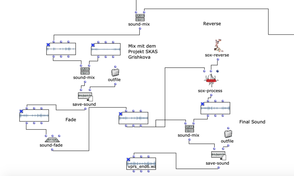
In der 6. Figur sieht man die letzte Bearbeitung. Ich mache einen Mix mit einem Audiomaterial (Mix 2 Sound + Takasugi) und meinem Projekt, welches ich im Rahmen von SKAS realisiert habe. Die Beschreibung des Projekts kann man hier finden.
Fg. 6 zeigt OpenMusic Patch „FinalMix“: Dieser Patch zeigt die letzte Transformation mit der Mono-spur
Das Ergebnis der letzen Iteration ist hier zu hören:
Dann habe ich die resultierenden Audio Dateien mit OMPrisma bearbeiten (s. Fig 7).
Hauptidee von Herrn Takasugi ist, dass Komponist (und Musiker) muss sehr persönlich Musik zu produzieren. Man muss „sich“ in der Komposition mitbringen.
Die Idee, dass Man „sich“ in der Komposition mitbringen muss, praktisch bedeutet aber auch, dass man irgendwelche zufällige Elemente mitbringt. Zufällige Elemente sind notwendig: als Menschen wir machen Fehler, wir können was übersehen, oder spontan entscheiden. Ich benutze OM-random um diese zufällige Elemente in der Komposition zu integrieren.
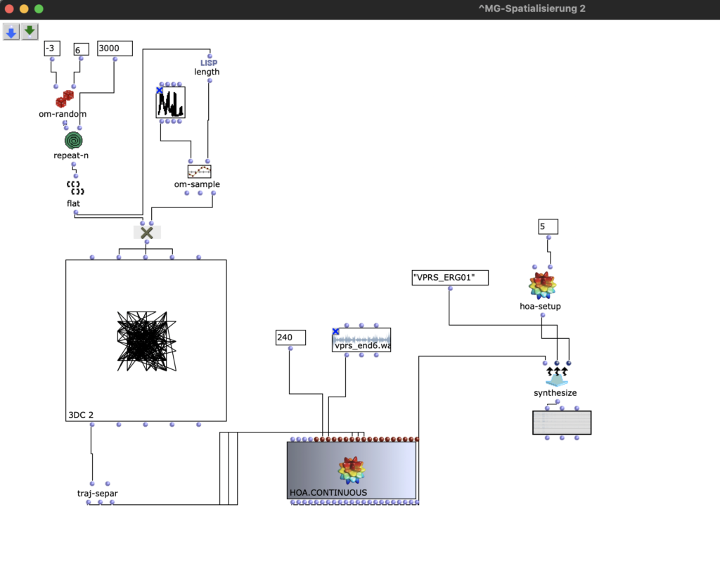
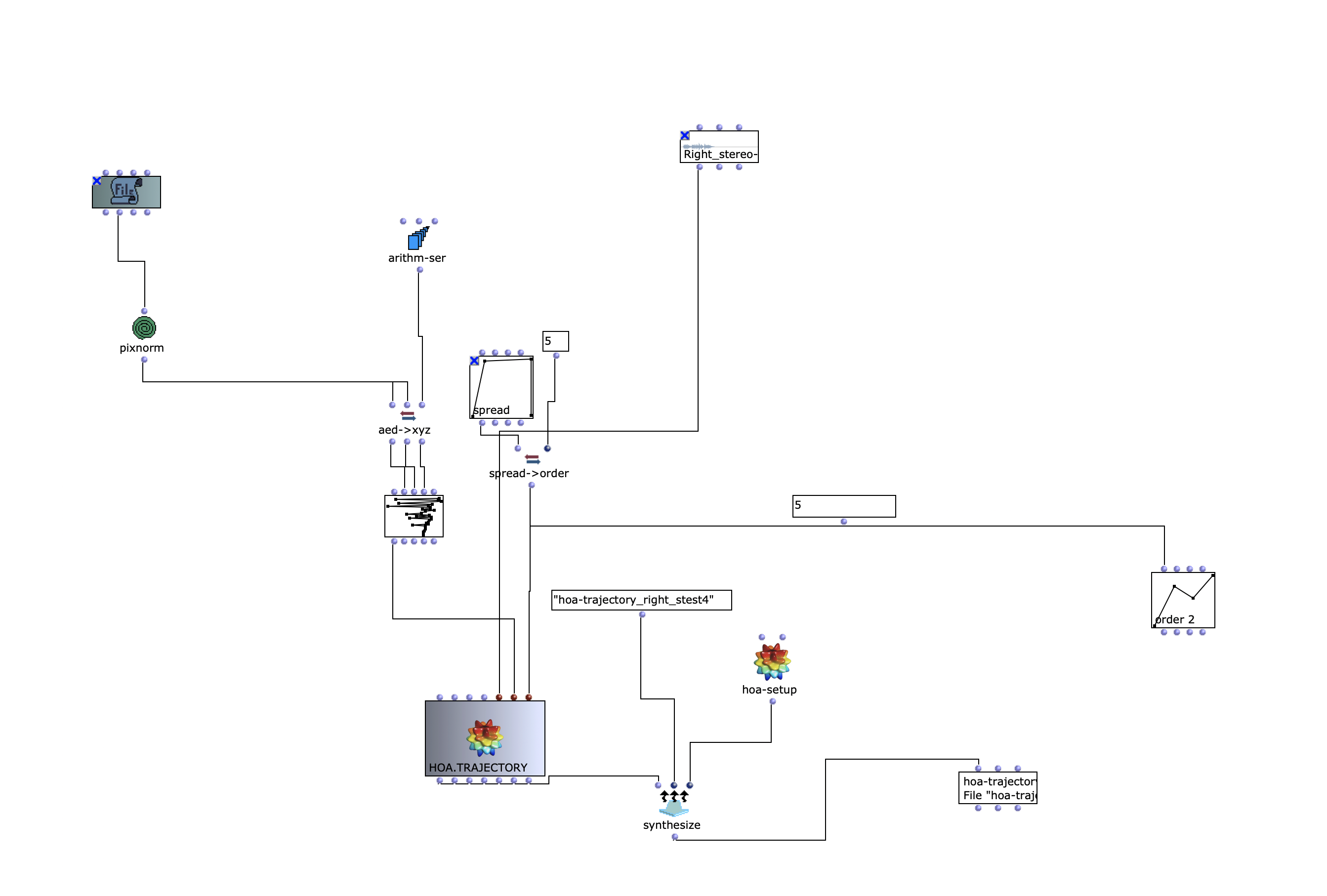
Fg. 7 zeigt OpenMusic Patch „OMPrisma“: Dieser Patch zeigt die Transformation mit HOA.Continuous
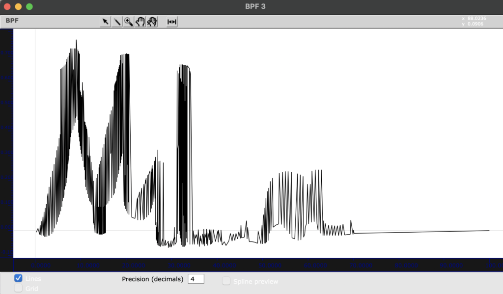
Als eine Methode um Komposition zu personifizieren benutze ich meine Name (Mila) als Muster für die Bewegung (s. Fig 8).
Fg. 8 zeigt OpenMusic Objekt „BPF“: Dieses Objekt zeigt mein Name als Muster für die Transformationen.
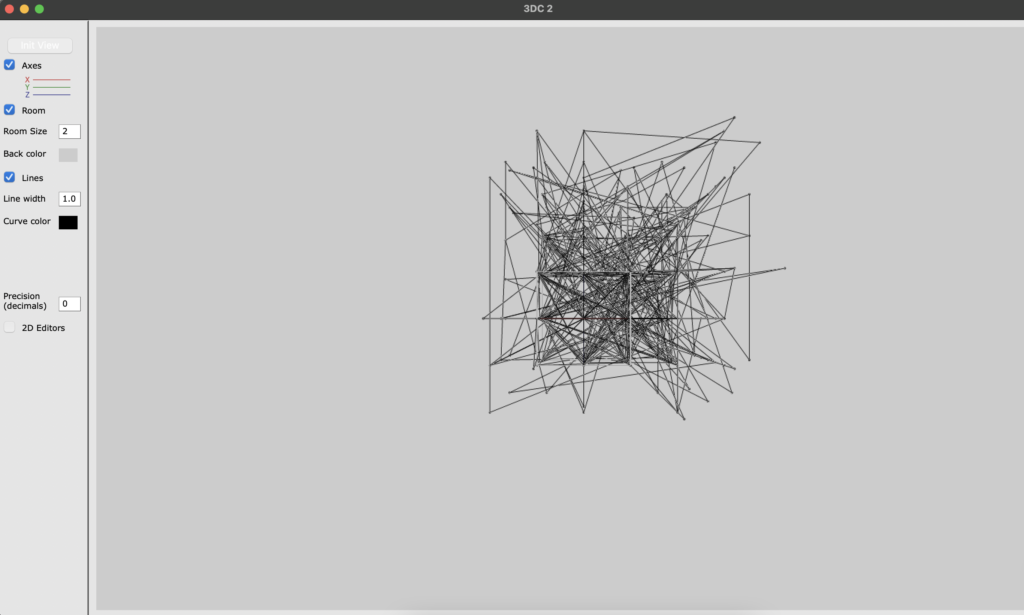
Dann benutze 3D OpenMusic Objekt. Mann kann auch 3D gut sehen (s. Fig. 9).
Fg. 9 zeigt OpenMusic Objekt „3DC“: Dieses Objekt zeigt die Transformationen.
Mit dem traj-separ Objekt kann man x-, y-, z- Koordinate nach HOA.Continuous schicken. Bei HOA.Continuous kann man auch die Länge der Komposition auszuwählen (im Sek). In meinem Fall steht 240, was 4 Minuten bedeutet.
Dann mit hoa-setup kann man auswählen, welche Klas von HOA man braucht. In meinem Fall ist HOA-setup 5, das bedeutet, dass ich High Order Ambisonic benutze.
Mann kann First Order Ambisonic und High Order Ambisonic unterscheiden. First Order Ambisonic ist eine Aufnahmemöglichkeit für 3D-Sound („First Order Ambisonic“ (FOA)), das aus vier Kanälen besteht und kann u.a. auch in verschiedene 2D-Formate exportiert werden (z. B. Stereo-, Surround-Sound).
Mit Ambisonic höherer Ordnung kann man Schallquellen noch genauer lokalisieren. Mann kann eine genauere Bestimmung des Winkels realisieren. Je höher die Ordnung, desto mehr Sphären kommen dazu.
„The increasing number of components gives us higher resolution in the domain of sound directivity. The amount of B-format components in High order Ambisonics (HOA) is connected with formula for 3D Ambisonics: (? + 1)2 or for 2D Ambisonics 2? + 1 where n is given Ambisonics order“. (C)
✅ Ergebnis OpenMusic Projekts mit OMPrisma kann man ? hier ? als Audio downloaded. ✅ Ergebnis OpenMusic Projekts mit OMPrisma kann man ? hier ? als Code downloaded.
✴✴✴✴✴✴✴✴✴✴✴✴✴✴✴✴✴✴✴✴✴✴✴✴✴✴✴✴✴✴✴✴✴✴✴✴✴✴✴✴✴✴✴✴✴✴
✅ Reaper
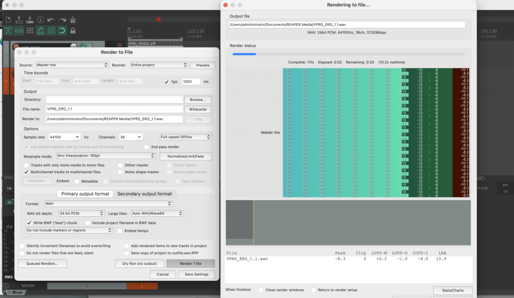
Dann habe ich die resultierenden Audio Dateien in ein Reaper Projekt importiert und die Ambisonics Audiospuren mit Plugins bearbeitet und neue Manipulationen gemacht.
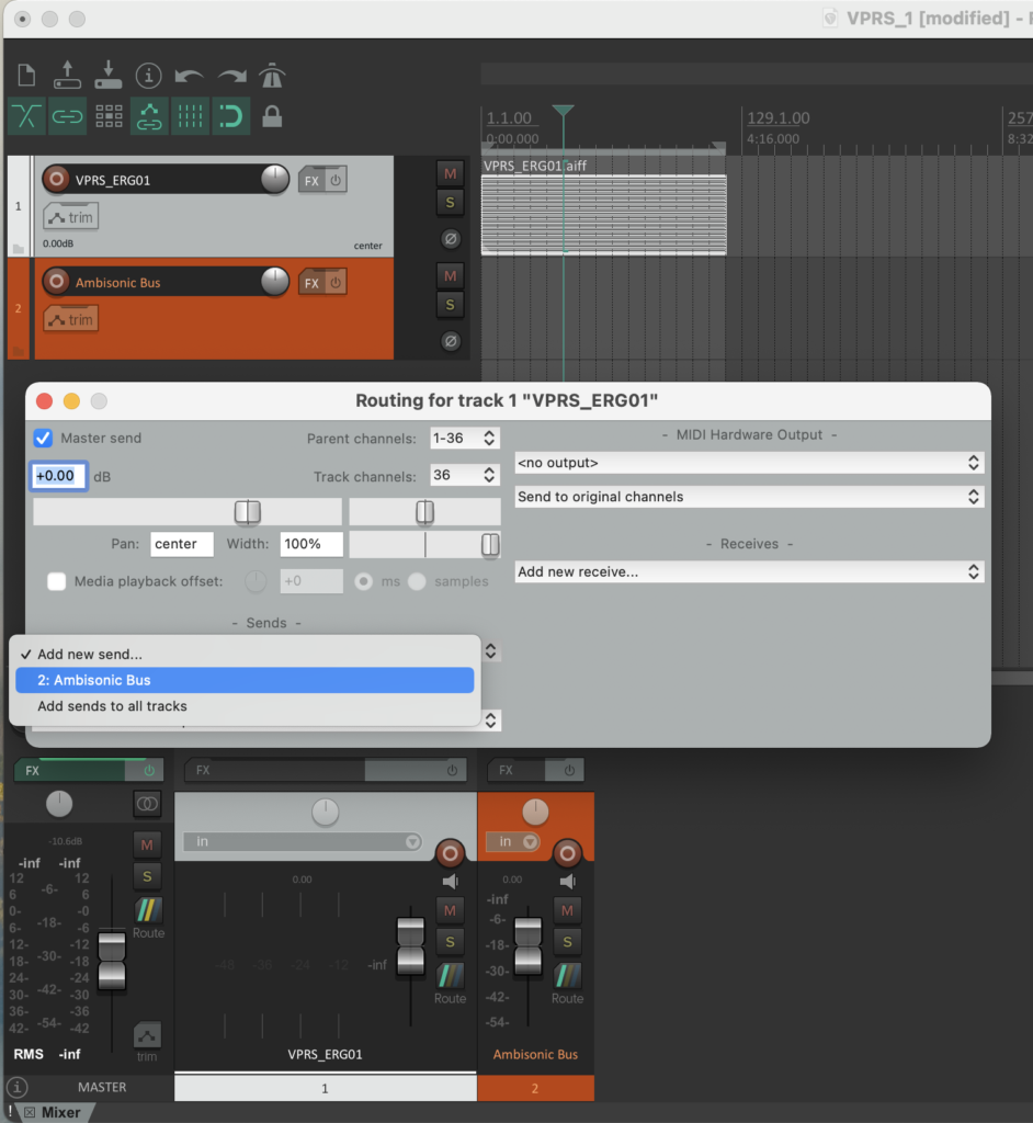
Nach dem das Audio material ist in Reaper hinzugefügt, muss man Routing machen. Hauptidee ist, dass 36 Kanäle werden beim ausgewählt und gesendet nach Ambisonic Buss (neuer Spur (s. Fig 10)).
Fg. 10 zeigt Reaper Projekt: Schritt Routing (36 Kanäle), sends nach Ambisonic Bus
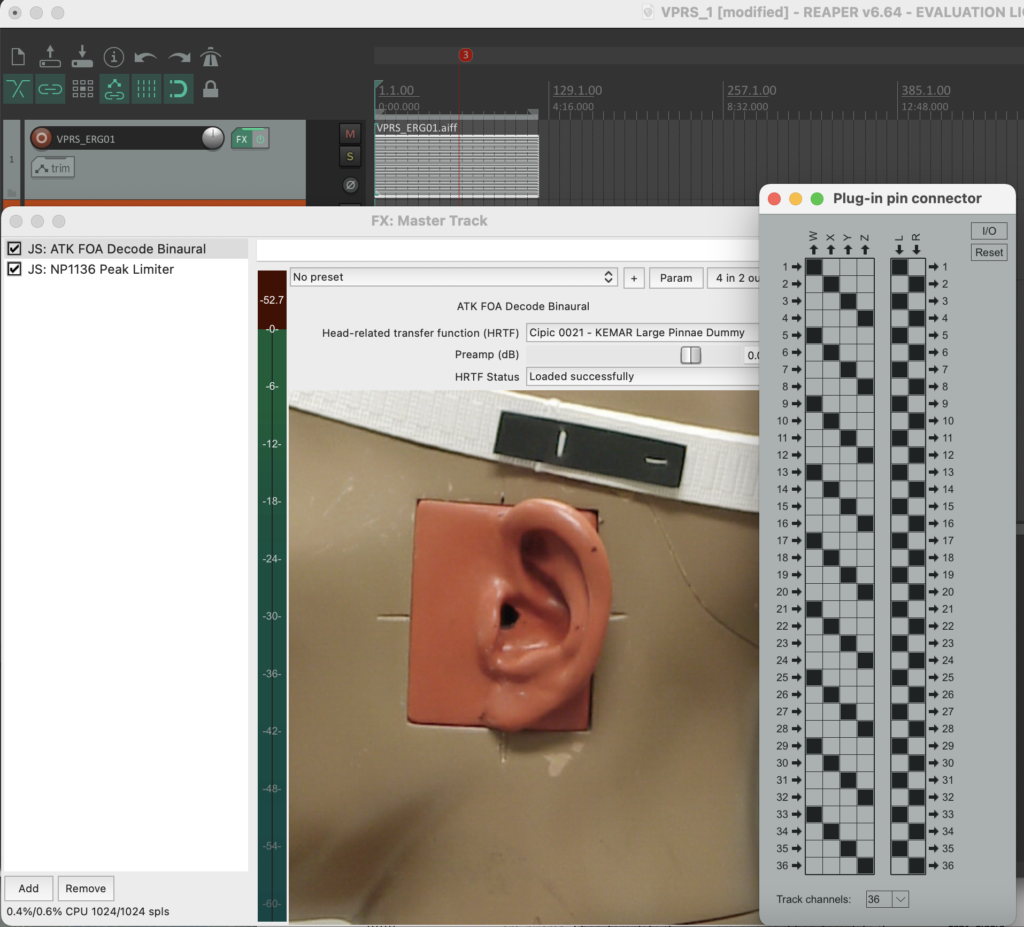
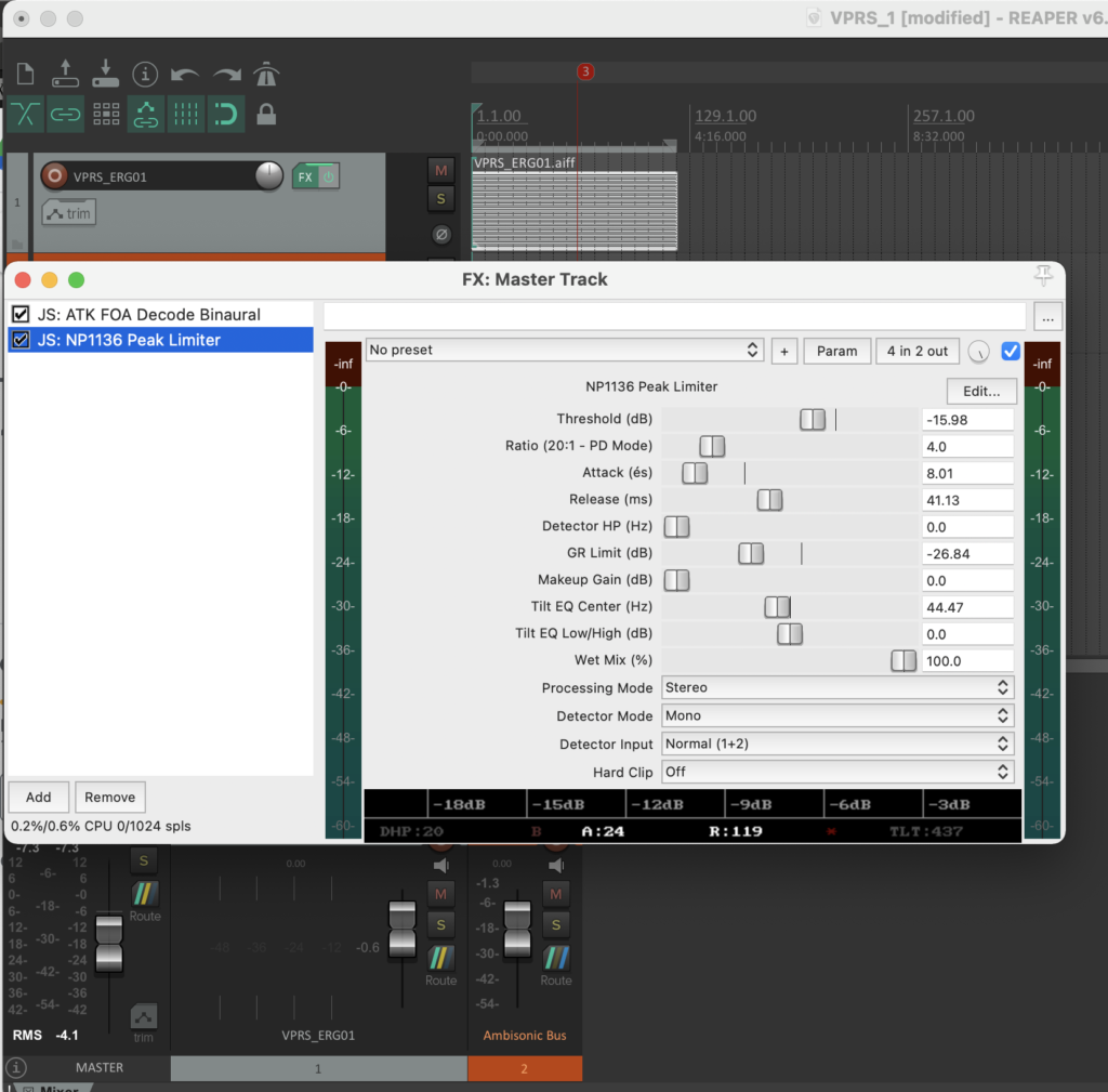
✅ Mixing & Plugins
Ich habe die Kodierung des vorbereiteten Materials in das B-Format gemacht, automatisierte dynamische spaialisieung verwendet habe. Ich habe auch dynamische Korrektur (Limiter) gemacht.
Mit Plugins kann man den Sound nach Belieben verändert und verbessert. In der Audiotechnik sind Erweiterungen für DAWs, auch die, die veschidene Instrumente simulieren, oder Hall und Echo hinzufugen. Die habe ich Reaper verwendet:
Dieser Beitrag handelt über die vierte Iteration einer akousmatischen Studie von Zeno Lösch, welche im Rahmen des Seminars „Visuelle Programmierung der Raum/Klangsynthese“ bei Prof. Dr. Marlon Schumacher an der HFM Karlsruhe durchgeführt wurden. Es wird über die grundlegende Konzeption, Ideen, aufbauende Iterationen sowie die technische Umsetzung mit OpenMusic behandelt.
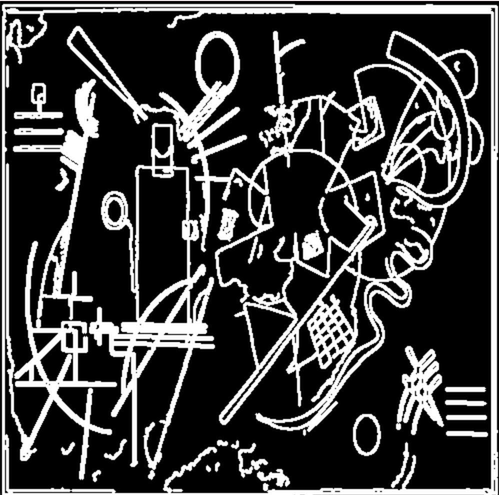
Um Parameter zum Modulieren zu erhalten, wurde ein Python-Script verwendet.
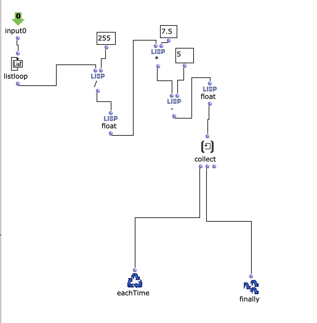
Dieses Script ermöglicht es ein beliebiges Bild auf 10 x 10 Pixel zu skalieren und die jeweiligen Pixel Werte in eine Text Datei zu speichern. „99 153 187 166 189 195 189 190 186 88 203 186 198 203 210 107 204 143 192 108 164 177 206 167 189 189 74 183 191 110 211 204 110 203 186 206 32 201 193 78 189 152 209 194 47 107 199 203 195 162 194 202 192 71 71 104 60 192 87 128 205 210 147 73 90 67 81 130 188 143 206 43 124 143 137 79 112 182 26 172 208 39 71 94 72 196 188 29 186 191 209 85 122 205 198 195 199 194 195 204 “ Die Werte in der Textdatei sind zwischen 0 und 255. Die Textdatei wird in Open Music importiert und die Werte werden skaliert.
Diese skalierten Werte werden als pos-env Parameter verwendet.
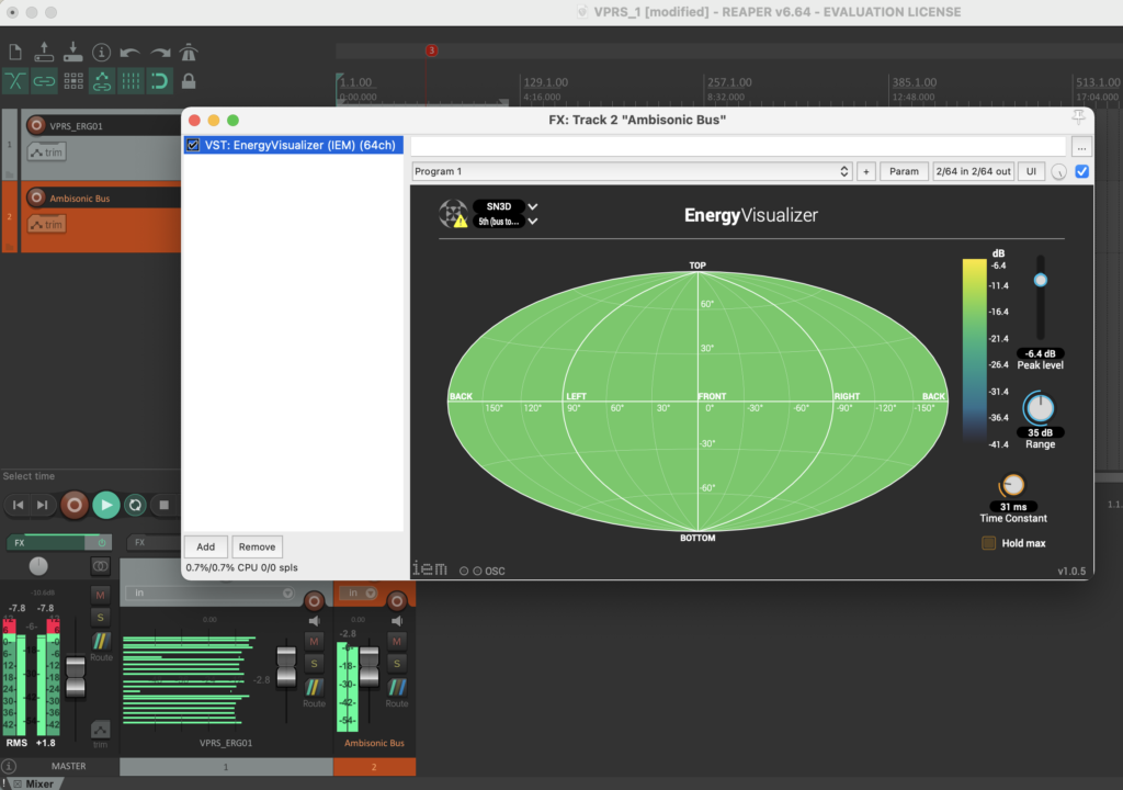
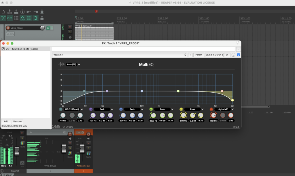
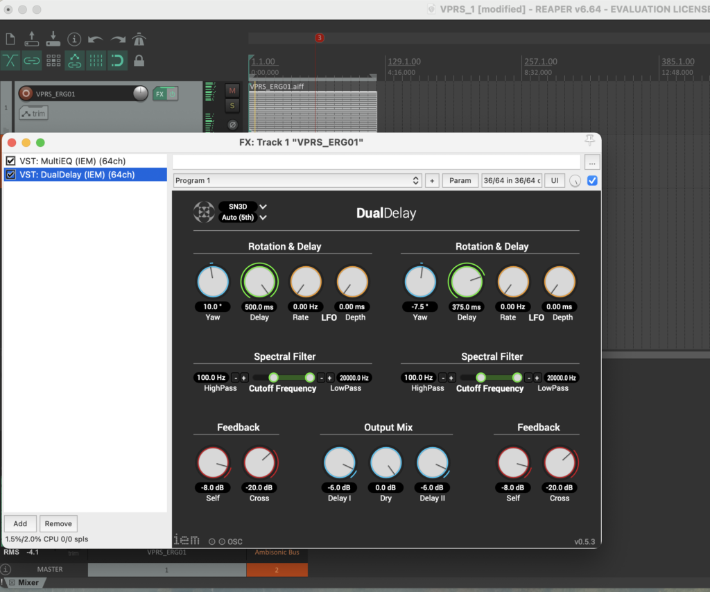
Reaper und IEM-Plugin Suite
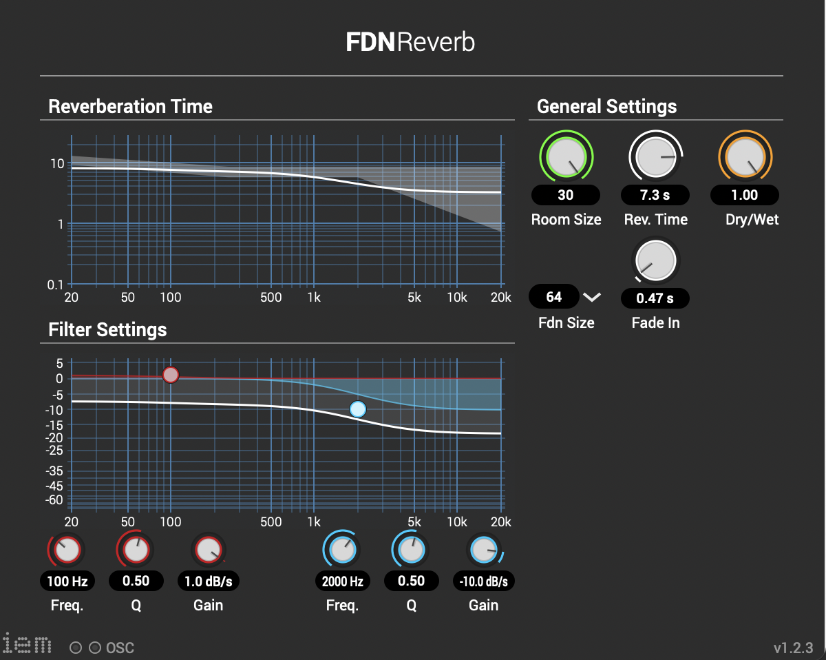
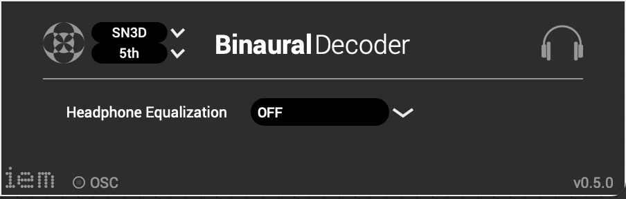
Mit verschiedenen Bildern und verschiedenen Skalierungen erhält man verschiedene Ergebnisse die für man als Parameter für Modulation verwenden kann. In Reaper wurden bei der Postproduktion die IEM-Plugin-Suite verwendet. Diese Tools verwendet man für Ambisonics von verschiedenen Ordnungen. In diesem Fall wurde Ambisonics 5 Ordnung angewendet. Ein Effekt der oft verwendet wurde ist der FDNReverb. Dieses Hallgerät bietet die Möglichkeit einen Ambisonics Reverb auf ein Mulikanal-File anzuwenden. Die Stereo und Monofiles wurden zuerst in 5th Order Ambisonics Codiert (36 Kanäle) und schließlich mit dem binauralen Encoder in zwei Kanäle umgewandelt. Andere Effekte zur Nachbearbeitung(Detune, Reverb) wurden von mir selbst programmiert und sind auf Github verfügbar. Der Reverb basiert auf einen Paper von James A. Moorer About this Reverberation Business von 1979 und wurde in C++ geschrieben. Der Algorythmus vom Detuner wurde von der HTML Version vom Handbuch „The Theory and Technique of Electronic Music“ von Miller Puckette in C++ geschrieben. Das Ergebnis der letzen Iteration ist hier zu hören.
Momentan umfasst die Library zwei Funktionen, die sowohl mit CommonLisp, als auch mit schon bestehenden Funktionen aus dem OM-Package geschrieben sind.
Zudem ist die Komposition im Umfang der zu kontollierenden Parametern, momentan auf die Harmonik und die Stimmführung begrenzt.
Für die Zukunft möchte ich ebenfalls eine Funktion schreiben, welche mit den Parametern Metrik und Einsatzabstände, die Komposition auch auf zeitlicher Ebene erlaubt.
Entwicklung: Lorenz Lehmann
Betreuung und Beratung: Prof. Dr. Marlon Schumacher
Mein herzlicher Dank für die freundliche Unterstützung gilt Joseph Branciforte und
I present in this article residual – i, a three-minute solo piece for prepared piano commissioned as a companion work to John Cage’s Sonatas and Interludes for prepared piano. In analyzing Cage’s work and subsequently composing a companion to it, I employed a self-designed texture synthesis tool driven by machine learning clustering. The technical overview of that tool can be read at this other blogpost, or in the proceedings of the 2022 International Conference on Technologies for Music Notation and Representation (TENOR 2022). The blogpost you are reading now will briefly explain how that tool (and generally, music informatics) was applied in composing this short piano piece.
Background
John Cage’s Sonatas and Interludes (1946-48) is a 60-minute work for solo prepared piano that involves placing various objects (metal screws, bolts, nuts, pieces of plastic, rubber and eraser) in the strings of the piano. These objects ‚prepare‘ the piano, altering its sound and bringing out a variety of different, heterogenous timbres. Some keys produce chords, others buzz, or even have the pitch completely removed. The sound profile of the Sonatas and Interludes are arguably the work’s most iconic aspect.
However, the form of the Sonatas and Interludes is also noteworthy. The work consists of sixteen sonatas and four interludes, with most movements lasting somewhere between 1 and 4 minutes each. As part of an ongoing commissioning project, pianist and composer Amy Williams premieres new ‚interludes‘ which are placed amidst the existing sonatas and interludes by Cage. In early 2022 I received the opportunity to compose a short piece that would use a piano with Cage’s „preparations“, and would be inserted as an interlude amidst the sonatas and interludes of Cage’s work.
Approach
I was interested in composing a piece that acknowledged both the sound- and time-identity of the Sonatas and Interludes. While arguably the most iconic aspect of Cage’s Sonatas and Interludes is its sounds, I feel that the work’s form, it’s time-based content, is equally impactful. Many of the its movements are cast in AABB form, reflecting classical period sonatas. Additionally, the distribution of the individual sonatas and interludes take a symmetrical form: four groups of four sonatas each, partitioned by the four interludes:
As a pre-compositional constraint, I decided that all sonorities in my piece would be taken/excerpted directly from the score of the Cage. To use the metaphor of a painter, the score of the Cage was my palette of colors, and not the prepared piano itself. This meant that not only every chord or single note in my piece would be excerpted from the Cage, it also meant that the chord or note’s particular duration would also be used in my piece. The sound and duration were joined as a single item. In a way, my piece was a form of granular synthesis, taking single-attack grains of the Sonatas and Interludes, and recontextualizing them in a new order.
Preprocessing
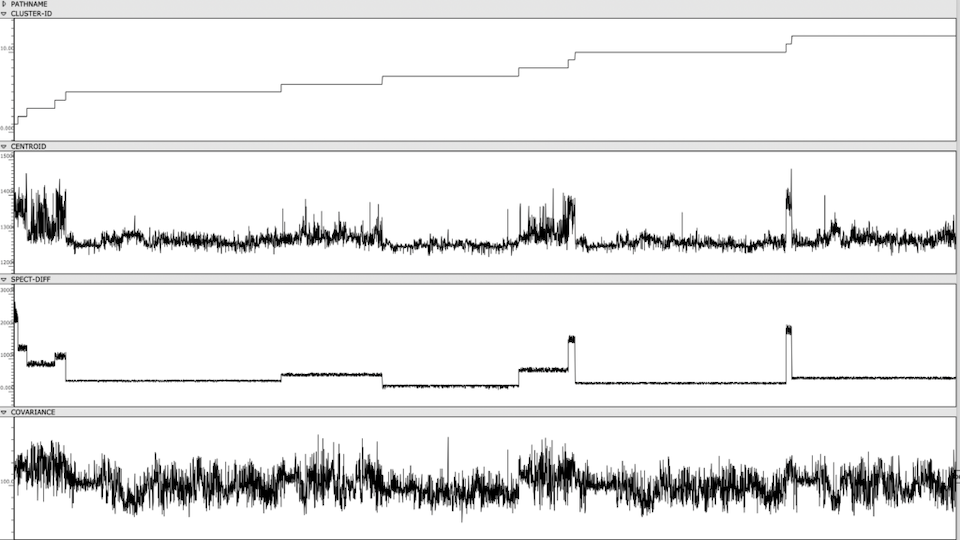
In order to observe and meaningfully comprehend all the individual sonorities in the 60-minute-long Cage, I used a simple machine learning clustering method to categorize all ~7k sonorities into 12 groups. Using my texture synthesis tool, I was not only able to organize audio features of these ~7k sonorities in a a visual editor, I was also able to export and listen to each individual sonority as a single, short audio file.
Figure 1: Clusters and audio features are visually represented and sorted, providing an out-of-time view of the Cage’s spectral content.
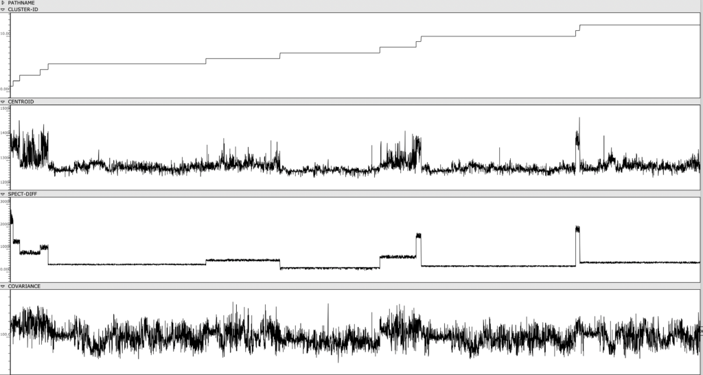
Once the sonorities have been extracted as individual transients, I used a k-means clustering method to sort these sonorities into 12 clusters. To briefly explain this machine learning method, the clustering algorithm receives a vector of several audio features as an input representing a sonority from the Cage (the audio features used were spectral centroid, spectral difference, and spectral covariance*). The algorithm then sorts these audio vectors into 12 groups, placing sounds with similar vector-values in the same group. This process in unsupervised, meaning it is not seeking to emulate a trained result that I predetermined. Rather, because these three audio features, as a trio, don’t represent any particularly given parameter in music, the algorithm returns clusters of sound that are correlated along multifaceted sound profiles that are aurally cohesive but not as simple as being sorted by a single parameter like pitch, duration, brightness, or noisiness.
Composition
My piece residual – i uses sonorities exclusively from clusters 2, 4, 9, 11. Referring back to the class-array figure, there is a clear line of differentiation between these clusters and the rest, correlated specifically to the spectral difference of the sonorities. These sonorities had an unusually high spectral difference, due either to their bright harmonic content (which creates a sharp delta between the attack and sustain of the transient) or their short duration (which creates a sharp delta between the attack and sustain/resonance of the transient). By placing each of these clusters in sequence, and the sounds within each cluster in sequence, this quality of shortness and brightness is clearly audible (see audio).
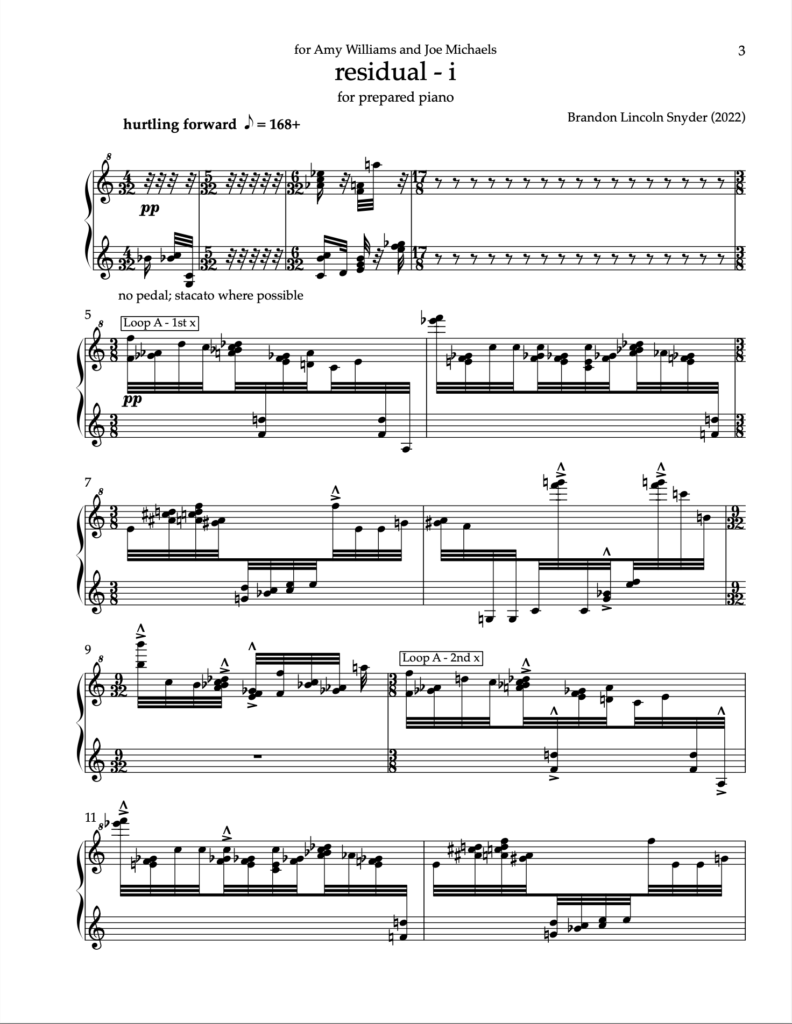
I treated this sequence as a kind of DNA for the piece. Large portions of it were copied into the score (sequences of around 20-30 transients. This process was done by hand, listening to each individual transient in the sequence, and looking up in the score of the Cage what the corresponding notes were). It was at this point that the machine learning methods involved in the piece are finished. From here, I began to sculpt and shape these longer sequences into shorter bursts. I also added repeat brackets at different moments, creating moments of ‚freeze‘ in the piece’s hurtling forward momentum.
Figure 3a: Loop A designates the first several (circa 20) sonorities in the cluster sequence, looped over and over. This sequence served as a scaffolding from which the piece was composed around.
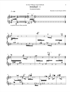
Figure 3b: This is the same page of the score, after notes have been removed, transforming the work into short bursts of sound.
Conclusion
Many of the cutting edge applications of machine learning in audio are towards the improvement of automated transcription, neural audio synthesis, and other tasks which have a clear goal and benchmark to test against. My particular application of machine learning in this piece is not for optimizing any task like this. Rather, the act of clustering audio served more as a means to explore the Sonatas and Interludes from a vantage point that I had not yet seen them from. Similar to my previous works that involve machine learning, being aware of how the machine learning methods are implemented is an essential first step in mindfully composing a work using such methods. As suggested by the title, residual – i serves as a proof of concept for a possible larger set of companion pieces, in which machine learning methods are used as a means to critically reexamine and „re-hear“ a familiar piece of music.
Listen to a full performance of residual – i here.
*These three features are measurements typically used to categorize the timbre and spectral content of an audio signal. The spectral centroid represents the center of mass in a spectrum. The spectral difference represents the average delta in energy between adjacent windows of the spectrum. The spectral covariance represents the spectral variability of a signal, i.e. how much the signal varies between its frequency bins.
Abstract: Beschreibung des elektromagnetischen Motion Tracking Systems G4 des Herstellers Polhemus und dessen Software
Verantwortliche: Prof. Dr. Marlon Schumacher, Daniel Fütterer
Das Polhemus G4 System erlaubt das Tracking von Positions- und Orientierungsdaten über magnetisch arbeitende Sensoren. Sender werden im Raum platziert und eingemessen/kalibriert, die Sensoren am zu messenden Objekt befestigt und an kabellose und tragbare Hubs angeschlossen. Diese übertragen die Daten an den PC, der wiederum diese Daten auswerten oder (wie in unserem Anwendungsfall) ins Netzwerk streamt.
Die Software des Herstellers läuft auf Windows und Linux, ist via kodiertem UDP-Export kompatibel mit der Spiele-Engine Unity und besteht jeweils aus mehreren Komponenten für Registrierung, Kalibrierung, Monitoring und Übertragung (z.B. mit Named Pipe oder UDP). Darüberhinaus sind große Teile der Software Open Source, was die Entwicklung individueller Tools ermöglicht.
Unter Linux gibt es eine Suite aus mehreren Programmen:
g4devcfg: Proprietäres Tool zur Konfiguration der Polhemus-Hardware (Dongle und Hub)
g4track_lib: Bibliotheken zur Verwendung mit den anderen Programmen
createcfgfile: Programm zur Erstellung der Config-Files (Aufstellung der Hardware)
g4display: Grafische Anzeige der Sensor-Position und -Orientierung
g4term: Textuelle Ausgabe der Sensor-Daten
g4export (Entwicklung von Janis Streib): Kommandozeilenprogramm zur Übertragung der Sensordaten via OSC
Angewendet wird die Software in Kombination mit Programmen wie Max/MSP oder PureData, die in der Lage sind, den OSC-Stream der Sensordaten auszulesen und zu verarbeiten.
Eine Beispielanwendung wird im Projekt des Studenten Lukas Körfer realisiert: Speaking Objects.


 Die Stereo und Monofiles wurden zuerst in 5th Order Ambisonics Codiert (36 Kanäle) und schließlich mit dem binauralen Encoder in zwei Kanäle umgewandelt.
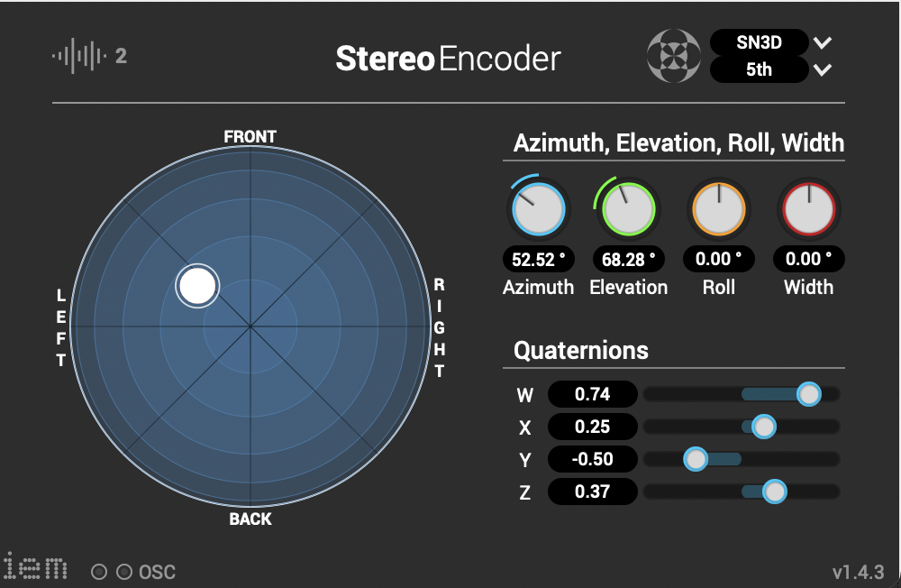
 Andere Effekte zur Nachbearbeitung(Detune, Reverb) wurden von mir selbst programmiert und sind auf Github verfügbar. Der Reverb basiert auf einen Paper von James A. Moorer About this Reverberation Business von 1979 und wurde in C++ geschrieben. Der Algorythmus vom Detuner wurde von der HTML Version vom Handbuch „The Theory and Technique of Electronic Music“ von Miller Puckette in C++ geschrieben. Das Ergebnis der letzen Iteration ist hier zu hören.